Zaher M.A. Alsulaiei*![]() | Hayder M. Hasan
| Hayder M. Hasan![]() | Mohsen H. Fagr
| Mohsen H. Fagr![]()
© 2025 The authors. This article is published by IIETA and is licensed under the CC BY 4.0 license (http://creativecommons.org/licenses/by/4.0/).
OPEN ACCESS
Heat exchangers (HE) are very imperative in numerous engineering, practical, and industrial fields because heat transfer (HT) and exchange is an important part of the operation of any heat machine, and special heat exchangers are needed to do so. The effectiveness of the heat exchanger is of great importance when studying the HT process inside the heat exchanger, as it determines the amount of heat transferred and is related to several things such as the type of working fluid, the size of the exchanger, its surface area, the flow rate, and many other factors. Adding nanomaterials at specific concentrations to the working fluids inside the heat exchangers improves the thermal properties of these fluids, which increases the efficiency of these exchangers. In this research, the effect of changing the volume fraction (VF) of graphene nanoparticles on the thermal performance of a parallel and counterflow tubular HE was studied using numerical modeling using Ansys Fluent 16.1 software. The results derived numerically were compared with with the analytical results to verify the validity of the solution. The results showed agreement with the analytical solution. The study showed that by increasing the VF of nanoparticles, the efficiency of the heat exchanger improves, whether the flow is parallel or counterflow. The numerical modeling results also showed an improvement in the NTU value with increasing the VF of nanoparticles.
exergy, economic cost, thermodynamics, ice thermal energy storage, objective function
Heat transfer (HT) is one of the basic sciences that a large number of researchers are still interested in in most engineering fields due to its importance in various aspects of life and many engineering applications [1].
Heat is transferred in three ways: Conduction, convection, and radiation. These methods are characterized by specific patterns in which one or two heat transfer methods may participate together to contribute to the total HT. Understanding the exact mechanism of each HT method and studying the method of heat transfer through different media has been of interest to a large number of researchers due to its importance in improving the investment conditions for many thermal systems, whether through maximum heat transfer or comprehensive insulation, which reduces heat transfer to its minimum [2].
Heat transfer by the three methods is a huge issue that is affected by many factors, such as the medium that transfers heat, the type of materials that contribute to heat conduction, the physical state of the material, and many variables and factors that affect heat transfer. When studying heat transfer, there are two prevailing methods: the experimental method and the analytical method, and each of the two methods has its preference under specific conditions and constraints. The number of researchers working with the analytical approach has increased with the numerical modeling of heat transfer equations, especially after the great development in the world of computing and the emergence of new generations of processors capable of solving millions of equations with millions of unknowns in a relatively short time, which prompted a large number of researchers to adopt the analytical approach and simulate computational fluid dynamics (CFD) in their research [3].
CFD is a modern science that is witnessing extensive development in many engineering fields due to the development of computer technology and the ability of new generations of processors to work efficiently in solving a large number of equations [4].
The addition of nanoparticles to the working medium in thermal devices improves the thermal properties of these devices. Many materials can be used and added to water, such as graphene, Al2O3, Ti, TiO2, Cu, Cuo, and other nanoparticles. As a result of the good thermal properties of these materials, they can raise the thermal properties of the nanofluid. Using graphene with water in particular increases the thermal conductivity (TC) of the new fluid because graphene has high TC. Therefore, adding graphene nanoparticles to water forms a fluid with high TC compared to water alone. It also improves the values of density, heat capacity, and other thermal properties associated with the new fluid [5].
The nanofluid produced by adding graphene to water in a specific volume ratio Has wide applicability in various engineering and heat-related fields, where it can be used in heat exchangers due to its major role in enhancing the heat transfer process. It is additionally suitable for applications involving heat pipes, sensors, refrigeration and air conditioning applications, lubrication, and other applications. Graphene-based nanofluid can be used in shell and tube heat exchangers (STE) to improve the efficiency of this type of exchanger [6].
Graphene nanofluids hold promise in high-performance, compact thermal systems, where maximizing heat transfer with minimal space and weight is critical. These systems include: Aerospace heat exchangers, microelectronics cooling systems, solar thermal collectors, high-efficiency heating, ventilation, and air conditioning (HVAC) systems, Automotive radiator applications.
The VF of nanoparticles Represents the ratio between the volume of nanoparticles and that of the entire fluid.
When studying a heat exchanger, we are dealing with the number of transfer units (NTU) rather than any non-dimensional number.
Bahmani et al. [7] studied heat transfer and turbulent flow of an aluminum oxide nanofluid in a double-pipe heat exchanger. The study showed that increasing the concentration of nanoparticles in the base fluid increased the heat transfer coefficient under both parallel and counterflow conditions. Rea et al. [8] demonstrated that using a nanofluid containing zirconium particles resulted in a 3% increase in the heat transfer coefficient, while the use of aluminum particles led to a 27% increase when heat transfer performance and pressure drop were assessed in a tube under laminar flow conditions. Das et al. [9] investigated the relationship between the temperature change of a nanofluid and the improvement of its thermal conductivity using Al₂O₃ and CuO. Goodarzi et al. [10] found that graphene exhibited the best thermal performance compared to other additives and was more economically preferable; the nanoparticles used in their study included Al₂O₃, graphene, Ti, TiO₂, Cu, and CuO. The effect of changing the type of nanoparticles added to water on the heat transfer coefficient and friction coefficient within a shell-and-tube exchanger was studied. Alawi et al. [11] experimentally investigated the energy efficiency of a flat-plate solar collector using graphene-based nanofluids (G-B-NFs), and the results showed an improvement in thermal properties and performance at constant heat flux. Ghozatloo et al. [12] conducted a thermodynamic evaluation (energy and exergy) of a shell-and-tube heat exchanger employing a graphene-based nanofluid, and demonstrated improved thermal performance under both laminar and turbulent flow conditions.
This research contributes to enhancing and improving the performance of heat exchangers by presenting a validated analytical-numerical methodology for solving them. While previous studies focused on numerical or experimental solutions, this methodology relied on both numerical and analytical solutions. The analytical and numerical results were compared to verify the validity of the numerical solution and provide a clear analytical methodology for studying shell-and-tube heat exchangers.
Also, most previous studies focused on aluminum, copper, and titanium oxides as nanomaterials added to the base fluid. However, this study used graphene as an additive, which is considered the least investigated nanomaterial when studying the thermal and hydraulic behavior of shell-and-tube heat exchangers. The study evaluates the effect of both nanoparticle VF and mass flow rate (MFR) on exchanger performance. This dual-criteria approach allows for a deeper understanding of operating conditions. The work utilizes a practical geometry (a shell-and-tube heat exchanger with realistic dimensions and boundary conditions), enhancing its relevance for industrial applications such as HVAC, process engineering, and power generation.
Following previous studies [13-16], this work employs a combined approach of numerical simulation using ANSYS software and conventional calculations to analyze heat transfer and fluid flow in a shell and tube HE using graphene-based nanofluid. The k-omega turbulence model will be used to evaluate flow and heat transfer inside the heat exchanger. Utilizing results from both ANSYS simulations and hands-on calculation methods for validation and comprehensive analysis [17].
The model is governed by several differential equations, which are solved using numerical approaches on the geometric model describing the rectangular finned channel. These equations include the equations of continuity, the momentum on the three axes (Navier-Stokes equations), the energy conservation equation, and the turbulence equations [10].
3.1 Continuity equation (conservation of mass)
The continuity equation describes the conservation of mass in a fluid flow system. It is expressed as follows [9]:
$\partial \rho / \partial t+\nabla \cdot(\rho u)=0$ (1)
where,
$\rho$ is the fluid density.
$t$ is time.
$u$ is the velocity vector.
$\nabla \cdot$ denotes the divergence operator.
3.2 Momentum equation (Navier-Stokes equation)
The equation describes the distribution of forces acting on the fluid and its motion. It is essentially Newton's second law applied to fluid motion. It is expressed as follows [12]:
$\rho\left(\frac{\partial u}{\partial t}+(u \cdot \nabla) u\right)=-\nabla p+\mu \nabla^2 u+f$ (2)
where,
$p$ is the pressure.
$\mu$ is the dynamic viscosity.
$\nabla^2$ is the Laplacian operator (a second-order differential operator).
$f$ is the external force vector per unit volume.
3.3 Energy equation
Conservation of energy in fluid flow systems is represented mathematically by the energy equation. It is based on the principles of thermodynamics and can be expressed as follows [3]:
$\rho\left(\frac{\partial E}{\partial t}+u \cdot \nabla E\right)=-\nabla \cdot(u(p+E))+\nabla \cdot(\kappa \nabla T)+\Phi$ (3)
where,
$E$ is the internal energy.
$\kappa$ is the TC.
$T$ is the temperature.
$\Phi$ is the dissipation function.
3.4 k-omega turbulence model
It Relies on two partial differential equations describing the distribution of turbulence kinetic energy (k) and specific dissipation rate (ω).
Turbulent Kinetic Energy (k) Equation: Describes the energy contained in turbulence [2].
$\frac{\partial k}{\partial t}+u_j \frac{\partial k}{\partial x_j}=\frac{\partial}{\partial x_j}\left[\left(v+\frac{v_t}{\sigma_k}\right) \frac{\partial k}{\partial x_j}\right]+P_k-\beta^* k \omega$ (4)
Specific Dissipation Rate (ω) Equation: Represents the rate of dissipation of turbulent kinetic energy per unit energy [4].
$\frac{\partial \omega}{\partial t}+u_j \frac{\partial \omega}{\partial x_j}=\frac{\partial}{\partial x_j}\left[\left(v+\frac{v_t}{\sigma_\omega}\right) \frac{\partial \omega}{\partial x_j}\right]+\alpha \frac{\omega}{k} P_k-\beta \omega^2$ (5)
where,
$v$: Kinematic viscosity.
$v_t$: Turbulent viscosity.
$\sigma_k, \, \sigma_\omega$: Prandtl numbers for k and ω.
$P_k$: Turbulent production term.
$\alpha, \, \beta, \, \beta^*$: Model constants.
It is preferred to use it for flows where wall effects significantly impact turbulence. Widely used in fluid flow analysis through wind tunnels or around smooth surfaces where wall effects are prominent [9].
3.5 Analytical procedure
Let us first determine the rate of heat capacity of the water flowing in both the shell and tube calculated from: $C_s=$ $\dot{m}_s . C_w, C_t=\dot{m}_t . C_w$, where $C_s$ is the average heat capacity of water in the shell, $C_t$ is the average heat capacity of water in the tube and $\dot{m}_s \dot{m}_t$ is the mass flow rate of water in both the tube and the shell respectively [6].
Calculation of the maximum heat transfer rate is performed through the following formula:
$\dot{Q}_{\max }=C_{\min }\left(\mathrm{T}_{\max , i \mathrm{n}}-\mathrm{T}_{\min , i n}\right)=C_t\left(\mathrm{~T}_{t, i n}-\mathrm{T}_{s, i n}\right)$ (6)
where, $T_{t, i n}$ and $T_{s, i n}$ are the water entry temperature in both the tube and the shell, respectively. Heat exchange surface area: $A=\pi D_{\text {inner}, t}. L$, where, $D_{\text {inner}, t}$ is the diameter of the inner tube and L is the length of the tube. The NTU is calculated as:
$N T U=\frac{U A}{C_{\min }}$ (7)
where, UA it is the total heat transfer coefficients (HTC) [18].
To calculate the total HTC, we have a fluid in the inner tube, which is hot water, the cylindrical wall of the inner tube, and the cold fluid, which is also water in the shell.
Heat is transferred from the hot fluid inside the inner tube to its inner surface through convection. Subsequently, conduction occurs across the wall of the inner tube to the outer surface. Finally, heat is transferred by convection from the outer surface of the inner tube to the cold fluid within the shell. It is essential to determine the convection HTC for both the tube and the shell, which depend on the Reynolds, Prandtl, and Nusselt numbers, as well as to evaluate the thermal resistance across the thickness of the inner tube the HTC by convection of the fluid in the inner tube ht calculated as [9]:
$h_t=\frac{N u_t \cdot K_t}{D_{\text {inner}, t}}$ (8)
where, $K_t$ is the thermal conductivity coefficient of the fluid within the inner tube [19]. $N u_t$ is the Nusselt number (NN) of the fluid in the inner tube and $D_{\text {inner}, t}$ is the diameter of the inner tube [20]. The NN is related to the Prandtl and Reynolds number, as it relates to the type of flow within the tube, whether it is turbulent or laminar, and this is related to the RN, and therefore the RN must be calculated for the fluid inside the tube as follow [6]:
$R e_t=\frac{\rho V_{m, t} D_{\text {Inner}, t}}{\mu}$ (9)
where, $V_{m,t}$ is the average velocity of flow in the inner tube and is calculated [2]:
$V_{m, t}=\frac{4 \cdot \dot{m}_t}{\rho \cdot \pi \cdot D_{\text {inner}, t}^2}$ (10)
We note that the RN is $3.10^3<R e<5.10^6$, and therefore the flow is turbulent, then the NN is calculated from the Gnielinski relation [4]:
$N u=\frac{\left(\frac{f}{2}\right)(R e-1000) P r}{1+12.7\left(\frac{f}{2}\right)^{0.5}\left(p r^{2 / 3}-1\right)}$ (11)
The coefficient of friction $f$ given by relation depending on the domain of the Reynolds number $10^4<R e_t<10^6$:
$f=\frac{1}{(1.58 \cdot \ln R e-3.28)^2}$ (12)
Let us now recalculate in order to determine the convection coefficient of the cold fluid moving within the shell, the value of the average velocity of flow in the shell calculated as:
$V_{m, s}=\frac{4 . \dot{m}_s}{\rho . \pi .\left(D_{\text {inner}, s}^2-D_{\text {outer}, t}^2\right)}$ (13)
where, $D_{\text {inner,} s}$ is the inner diameter of the shell, and $D_{\text {outer,} t}$ is the outer diameter of the tube. Thus, the RN of the fluid within the shell can be calculated from the relationship [7]:
$R e_s=\frac{\rho \cdot V_{m, s} \cdot D_{h y d}}{\mu}$ (14)
where, $D_{h y d}$ is the hydraulic diameter of the annular space of the shell and is given by the relation [6]:
$\begin{gathered}D_{\text {hyd }}=4 \frac{A_{\text {flow }}}{\prod}=\frac{4 \cdot \frac{\pi}{4}\left(D_{\text {inner}, s}^2-D_{\text {outer}, t}^2\right)}{\pi\left(D_{\text {inner}, s}+D_{\text {outer}, t}\right)}=D_{\text {inner}, s}-D_{\text {outer}, t}\end{gathered}$ (15)
where, $A_{\text {flow }}$ represents the cross-sectional area of the flow and $\prod$ represents the wetted perimeter.
Therefore, this flow is turbulent, and therefore the friction coefficient and NN is calculated from the same previous relationship based on hydraulic diameter.
The HTC due to convection in the fluid in the shell is then considered:
$h_s=\frac{K_s N u_s}{D_{h y d}}$ (16)
Now the overall HTC is determined by the relationship [3]:
$\frac{1}{U A}=R=R_i+R_{\text {wall}}+R_o$ (17)
$R_i$ and $R_o$ represent the convection thermal resistance of the internal and outer fluid respectively and given by:
$R=\frac{1}{h_s \cdot A}$ (18)
$R_{wall}$ represents the thermal resistance of the inner wall of the tube and is given by:
$R_{\text {wall }}=\frac{\ln \left(\frac{D_{\text {outer}, t}}{D_{\text {inner}, t}}\right)}{2 \pi K_{\text {wall}} L}$ (19)
$K_{wall}$ represents the TC of the inner wall material. Substitute in the relation for the total HTC [2]:
$R=\frac{1}{U A}=\frac{1}{\pi L}\left(\frac{1}{h_t D_{\text {inner}, t}}+\frac{\ln \left(\frac{D_{\text {outer}, t}}{D_{\text {inner}, t}}\right)}{2 K_{\text {wall}}}+\frac{1}{h_s D_{\text {outer}, t}}\right)$ (20)
The heat capacity ratio is given by:
$c=\frac{c_{\text {min}}}{c_{\text {max}}}=\frac{c_t}{c_s}$ (21)
The effectiveness of the STE with parallel and counter flow is calculated according to the relationship [18]:
$\varepsilon_{\text {parallel}}=\frac{1-e^{\left[-\frac{U A}{C_{\min}}\left(1+\frac{c_{\min}}{c_{\max}}\right)\right]}}{1+\frac{c_{\min}}{c_{\max}}}$ (22)
$\varepsilon_{\text {counter }}=\frac{1-e^{\left[-\frac{U A}{C_{\min }}\left(1-\frac{c_{\min }}{c_{\max }}\right)\right]}}{1-\frac{c_{\min }}{c_{\max }} e^{\left[-\frac{U A}{c_{\min }}\left(1-\frac{c_{\min }}{c_{\max }}\right)\right]}}$ (23)
For the VF of nanographene 0.005 by substituting into the previous relationships the effectiveness values of the heat exchanger are $\varepsilon_{\text {parallel }}=0.172$ and $\varepsilon_{\text {counter }}=0.174$.
3.6 Case study
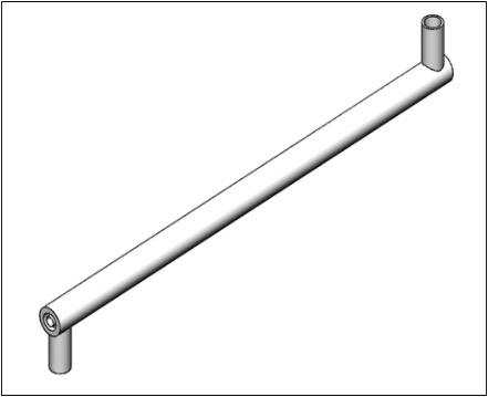
In this paper, we will use a stainless-steel heat exchanger with parallel and counter flow, and the heat transfer process will take place between the hot fluid flowing in the inner tube and the cold fluid moving in the outer shell, as in Figure 1 and Table 1 showed these dimensions [20, 21]. The basic operating conditions for this exchanger are shown in Table 2. The physical properties of materials used are shown in the Table 3.
Table 1. Dimensions of heat exchanger
|
Heat Exchanger |
Inner Tube (t) |
Annular Shall (s) |
|
Inner diameter Dinner(m) |
0.015 |
0.032 |
|
Outer diameter Dinner(m) |
0.019 |
0.052 |
Figure 1. Geometry of shell and tube
Table 2. Operation condition
|
Operation Conditions |
Inner Tube |
Outer Shell |
|
Water mass flow rate Kg/s |
0.2 Kg/s |
0.8 Kg/s |
|
Entry temperature K |
343.2 Kg/s |
283.2 Kg/s |
Table 3. Physical properties for materials
|
Physical Prosperities |
Stainless Steel |
Water (Based Fluid) |
Graphene Nanoparticles |
|
Density ($\rho$) |
8100 |
998.2 |
2250
|
|
Heat Capacity ($C_p$) |
Vary Linearly with temperature |
4182 |
710
|
|
Thermal conductivity ($K$) |
Vary Linearly with temperature |
0.6 |
2000 |
|
Viscosity ($\mu$) |
---- |
0.001003 |
------ |
The analytical method will first be used to calculate the temperature at the outlet of the exchanger for the inner tube into which the hot water enters by using the NTU method of the shell-and-tube heat exchanger, and then compare the analytical result with the modeling results to validate the results. The properties of the nanofluid are calculated from the relationships [17]:
$\begin{gathered}\rho=(1-\varphi) \rho_w+\varphi \rho_{n p} \\ C_p=\frac{(1-\varphi) \rho_w C_{p w}+\varphi \rho_{n p} C_{p n p}}{(1-\varphi) \rho_w+\varphi \rho_{n p}} \\ K=\frac{k_w\left[k_{n p}+(n-1) k_w-(n-1) \varphi\left(k_w-k_{n p}\right)\right]}{k_{n p}+(n-1) k_w+\varphi\left(k_w-k_{n p}\right)} \\ \mu=\mu_w(1+2.5 \varphi)\end{gathered}$ (24)
where, the suffix np stands for the properties of nanoparticles and the suffix w for water, but without the suffix, it is the properties of nanofluids. (Volume Fraction): It is the ratio of the volume occupied by nanoparticles to the total volume of the nanofluid. Graphene particles take the shape of flakes rather than the spherical shape. Therefore, when applying the Hamilton and Croser equation in the TC coefficient equation, a value of the particle shape coefficient n=1.14 must be used [22].
4.1 CFD simulation
The numerical modeling process includes firstly describing the studied geometric model that represents the volume of the fluid within the studied channel, then forming the mesh and studying its independence from the numerical solution, and then determining the physical properties of the working fluid and the boundary conditions necessary to solve the mathematical model.
In this modeling, the effectiveness of the parallel and counterflow heat exchanger was studied at graphene VF in water of 0.001, 0.003, 0.005, 0.007 and 0.009. The solution was verified and the temperature contours within the shell and tube were shown at a graphene VF of 0.005.
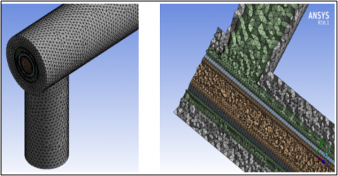
In this paper, tetrahedral cells were generated for ease of generation in the Ansys meshing software, as in the attached Figure 2, which show the cells in general, and a section was formed to show the shape of the cells from inside the model.
Figure 2. The mesh of heat exchanger
To capture the gradient in Temperature and Velocity near the wall boundaries zone, inflation layer was introduced as in Figure 2 on the right.
Table 4. Mesh independence study
|
Elem Size |
No. of Cells |
NTU |
|
3 |
90000 |
0.159 |
|
2 |
150000 |
0.168 |
|
1 |
400000 |
0.172 |
|
0.5 |
1180000 |
0.179 |
|
0.25 |
2883670 |
0.179 |
Table 5. Boundary condition
|
Region |
Boundary Conditions |
|
Inner tube fluid |
MFR and Temperature |
|
inner shell fluid |
MFR and Temperature |
|
Inner tube |
Surface Interface Coupled |
|
Outer shell |
Surface interface Coupled Adiabatic outer surface |
|
Exit shell and tube |
Pressure outlet (Zero gage pressure) |
A mesh study concept is the analysis of the impact of mesh size and distribution on the accuracy of numerical simulation results. It is an essential step in ANSYS to ensure a balance between result accuracy and computational costs. A mesh study was conducted using five different values and the number of the cells specified in Table 4. In order to solve the proposed mathematical model, which is a set of partial differential equations, it is necessary to determine the boundary conditions necessary to solve these equations. These conditions are shown in Table 5.
4.2 Discussion
To solve the primary flow equations while coupling velocity, pressure, and temperature, the software employs various algorithms to ensure solution convergence. The SIMPLE scheme is selected for pressure-velocity coupling, utilizing second-order interpolation for all variables. The fundamental equations—including continuity, momentum, energy, and the turbulence model—are discretized algebraically using a second-order scheme. This approach balances solution accuracy with reduced computational effort compared to higher-order discretization methods. Convergence criteria are defined based on the residuals of all flow equations, requiring them to fall below predefined thresholds (e.g., a specific limit for the continuity equation and slightly different limits for the other equations).
In order to verify the correctness of the solution, we calculate the temperatures at the cold and hot outlet of the exchanger numerically and then calculate the effectiveness values from the relationship,
$\varepsilon=\frac{T_{\max,{in}}-T_{\max,{out}}}{T_{\max.{in}}-T_{\min,{in}}}=\frac{T_{t,{in}}-T_{t,{out}}}{T_{t,{in}}-T_{s,{in}}}$ (25)
where, the effectiveness values for the parallel and countercurrent flow calculated numerically are $\varepsilon_{\text {parallel }}=$ 0.1601 and $\varepsilon_{\text {counter }}=0.1608$ respectively, i.e. with a relative error of approximately $6.9 \%$ for the parallel flow and $7.5 \%$ for the countercurrent flow, which is an acceptable error compared to the analytical results.
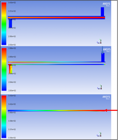
Figure 3 shows the temperature contours within the exchanger, the shell and the tube in the case of parallel flow, where the temperature value calculated as an area weighted average at the tube outlet is 333.59 K and at the shell outlet is 286.35 with an effectiveness of 0.1601. The thermal gradient can be observed in this case within the tube, while in the shell we notice that the upper part is hotter than the lower part as a result of the vortex motion of the fluid within it, which contributes to the transfer of hot currents upwards.
Figure 3. Parallel flow heat exchanger temperature contours
Figure 4. Counter flow heat exchanger temperature contours
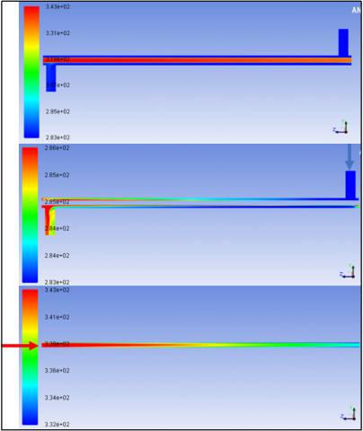
Moving to the counterflow case, the Figure 4 shows temperature contours within the exchanger, shell and tube, where we notice a thermal behavior similar to the parallel flow case with the opposite direction of the temperature gradient within the tube as a result of the change in the flow direction within the tube. The temperature value when calculated as an area weighted average at the tube outlet is 333.52 K and at the shell outlet is 286.34 with an effectiveness of 0.1608.
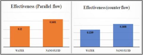
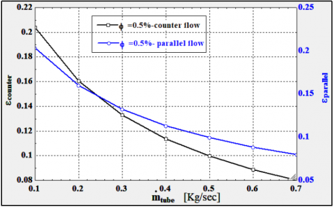
By comparing the temperature and effectiveness values in the Table 6 in the parallel and counterflow cases when using graphene-based nanofluid with the parallel and counterflow cases when using water only as a heat exchange medium, we notice an increase in the effectiveness of the exchanger in the parallel flow case by 33.4% when using graphene nanofluid, while this effectiveness increases by only 33% in the counterflow case as is clear from the Figure 5. For a VF of graphene of 0.005, the change in effectiveness can be studied with varying flow rate in the tube and the flow rate in the shell remaining constant as shown in the Figure 6.
Table 6. Comparing the temperature and effectiveness values
|
|
Nano Fluid with 0.005 Graphene Volume Fraction |
Water |
||
|
|
Parallel flow |
Counter flow |
Parallel flow |
Counter flow |
|
T-t, outlet |
333.59 |
333.51 |
336 |
336.1 |
|
T-t, outlet |
286.35 |
286.34 |
285 |
285.21 |
|
Effectiveness |
0.1601 |
0.1608 |
0.12 |
0.1209 |
Figure 5. Effectiveness values
Figure 6. Effectiveness VS mass flow rate in tube
Graphene exhibits exceptionally high TC. (approximately 2000 W/m·K), much higher than that of water (approximately 0.6 W/m·K). When dispersed in water, even in small volumetric proportions, graphene forms heat-conducting pathways through the core fluid, allowing for faster transfer of thermal energy between hot and cold regions. This results in steeper temperature gradients and faster energy dissipation, improving heat exchanger efficiency. The presence of nanoparticles also increases the effective TC and alters the thermophysical properties of the fluid (such as viscosity, density, and specific heat), which in turn increases the NN. Increased turbulence near the boundary layers also enhances convective heat transfer, especially under turbulent flow.
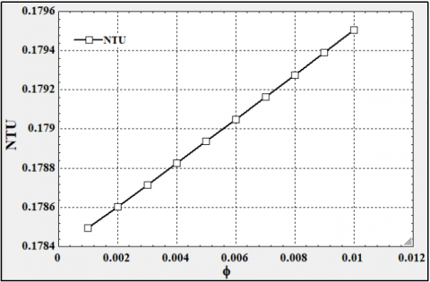
We notice that the more the flow rate increases within the tube while the flow within the shell is constant, Effectiveness in heat exchange operations, whether the flow is parallel or counter, decreases. This is due to a decrease in the NTU value as a result of the increase in the thermal capacity rate, as the fluid must remain within the tube in order to be able to exchange heat with the shell. Consequently, the increase in flow rate causes an increase in the speed of the fluid inside the tube and thus reduces its residence time within the tube. This explains the decrease in the effectiveness value. Adding nanomaterials with high thermal properties to water improves, as we mentioned earlier, the thermal properties of water, making it a fluid with high TC. Consequently, we notice an increase in the value of the number of HT units NTU due to the increase in the thermal convection coefficient in the nanofluid and the decrease in its thermal capacity value. The more the VF of the nanomaterial within the fluid increases, the more the NTU value of the working medium increases due to the greater improvement in thermal properties. The Figure 7 shows the increase in the NTU value of the nanofluid within the heat exchanger as the VF of graphene increases in it.
Figure 7. Volume fraction of nano-graphene VS NTU
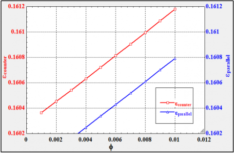
Figure 8. Effectiveness VS volume fraction of graphene
Certainly, the increase in NTU values as a result of the increase in the VF of the graphene nanomaterial will cause an increase in the heat exchanger effectiveness value, whether the flow is parallel or counterflow. The Figure 8 shows the change in the effectiveness value as the VF of graphene in the water increases.
We note that doubling the VF from 0.005 to 0.01 leads to an increase in effectiveness from 0.1601 to 0.1608 in parallel flow, i.e., by 0.43%, and an increase in effectiveness from 0.1608 to 0.1612 in counterflow, i.e., by 0.24%. This indicates the uneconomically of increasing the concentration of the nanomaterial dispersed within the water in order to increase the thermal effectiveness within the heat exchanger.
Higher MFR in the inner tube result in higher RN, which are typically associated with better HT. However, this comes at the expense of reduced residence time within the exchanger. As a result, despite the higher convection coefficient, the fluid has less time to absorb or release heat, reducing the overall efficiency (ε). This explains why the efficiency decreases as the flow rate increases while maintaining constant flow along the shell, as confirmed by the numerical results.
Increasing the volumetric fraction of graphene improves TC and, consequently, the NTU. However, beyond a certain concentration (e.g., 0.005-0.01), the gain in NTUs becomes marginal, while increasing viscosity may increase pumping force and the potential for clogging or fouling. Therefore, from an energy and economic perspective, there is a diminishing return at higher concentrations.
Adding nanoparticles slightly increases the viscosity of the fluid, especially at higher concentrations. This results in increased flow resistance and pressure drop, which must be taken into account when designing the system. However, within the tested range (up to 0.009 volume fraction), the increase in viscosity is moderate and does not significantly affect flow characteristics. In short, the optimization mechanisms primarily rely on improving the conductivity and convection properties of the nanofluid, while taking into account fluid dynamic constraints such as residence time and increased viscosity.
This work not only confirms the thermal benefits of graphene-enhanced nanofluids but also provides a validated practical framework for their application in industrial heat exchangers. Future work may include experimental validation and lifecycle cost analysis to further guide deployment strategies.
4.3 Environmental and economic consideration
Beyond thermal analysis, the study goes a step further by assessing the economic practicality of increasing nanoparticle VF. It finds diminishing returns at higher concentrations, providing insight into the cost-effectiveness trade-off a point often overlooked in purely thermal-focused research.
While graphene nanoparticles significantly improve the thermal performance of aqueous fluids in heat exchangers, their economic viability remains a major concern. Graphene production, especially in high-purity flakes and fixed flakes suitable for nanofluid applications, remains relatively expensive compared to other nanoparticles such as Al₂O₃ or TiO₂. The slight improvement in efficiency observed above a volume fraction of 0.005 (only about 0.43% in parallel flow) indicates diminishing returns with increasing concentration. Therefore, an optimal balance must be achieved between performance improvement and cost of nanoparticles, especially in large-scale applications where operating cost is a critical factor [17].
The environmental impacts of using graphene-based nanofluids are not yet fully understood, particularly with regard to release of nanoparticles into ecosystems during disposal or leakage and Bioaccumulation and toxicity of graphene particles in aquatic systems.
To mitigate these risks, strict handling and disposal regulations and the use of closed-loop fluid systems are recommended. Furthermore, research into biodegradable or less hazardous surfactants and stabilizers for graphene emulsions could contribute to improved environmental safety [4].
Heat exchangers play a major character in many industrial and thermal applications, so increasing the effectiveness of HT within these exchangers is a necessary requirement.
A dual approach combining NTU-based analytical modeling and computational fluid dynamics (CFD) simulation using ANSYS Fluent was used. The high degree of agreement (within 7.5% relative error) confirms the validity of the numerical model and supports its application in further parametric studies. The effectiveness of heat exchange in these exchangers can be increased by adding nanomaterials to the working medium in specific concentrations, as this contributes to enhancing the thermal properties of this working medium. Numerical modeling shows agreement between the analytical solution for the STE and the numerical solution, which allows studying these exchangers in more detail using numerical modeling techniques. Adding nano-graphene to water with a VF of 0.005 in the STE increases its heat exchange effectiveness by 33.4% in the case of parallel flow and by 33.2% in the case of counterflow. Increasing the VF of graphene in water within the STE increases its thermal efficiency, but by 0.43% for parallel flow and 0.24% for counterflow, so this increase is not desirable from an economic point of view.
The study identifies an inverse relationship between the flow rate on the tube side and the efficiency of the heat exchanger, due to the reduced fluid residence time. This insight is crucial for improving operating conditions in practical systems. The slight improvement in performance at higher VF (above 0.005) highlights the economic limitations of excessive use of nanoparticles. These results encourage the practical and effective Use of nanofluids in industrial heat exchanger systems.
[1] Ding, Y., Alias, H., Wen, D., Williams, R.A. (2006). Heat transfer of aqueous suspensions of carbon nanotubes (CNT nanofluids). International Journal of Heat and Mass Transfer, 49(1-2): 240-250. https://doi.org/10.1016/j.ijheatmasstransfer.2005.07.009
[2] Balandin, A.A., Ghosh, S., Bao, W., Calizo, I., Teweldebrhan, D., Miao, F., Lau, C.N. (2008). Superior thermal conductivity of single-layer graphene. Nano Letters, 8(3): 902-907. https://doi.org/10.1021/nl0731872
[3] Novoselov, K.S., Geim, A.K., Morozov, S.V., Jiang, D.E., et al. (2004). Electric field effect in atomically thin carbon films. Science, 306(5696): 666-669. https://doi.org/10.1126/science.1102896
[4] Stankovich, S., Dikin, D.A., Piner, R.D., Kohlhaas, K.A., et al. (2007). Synthesis of graphene-based nanosheets via chemical reduction of exfoliated graphite oxide. Carbon, 45(7): 1558-1565. https://doi.org/10.1016/j.carbon.2007.02.034
[5] Bahaya, B., Johnson, D.W., Yavuzturk, C.C. (2018). On the effect of graphene nanoplatelets on water–graphene nanofluid thermal conductivity, viscosity, and heat transfer under laminar external flow conditions. Journal of Heat Transfer, 140(6): 064501. https://doi.org/10.1115/1.4038835
[6] Jiji, L.M., Danesh-Yazdi, A.H. (2009). Heat Conduction (Vol. 3). Berlin: Springer.
[7] Bahmani, M.H., Sheikhzadeh, G., Zarringhalam, M., Akbari, O.A., Alrashed, A.A., Shabani, G.A.S., Goodarzi, M. (2018). Investigation of turbulent heat transfer and nanofluid flow in a double pipe heat exchanger. Advanced Powder Technology, 29(2): 273-282. https://doi.org/10.1016/j.apt.2017.11.013
[8] Rea, U., McKrell, T., Hu, L.W., Buongiorno, J. (2009). Laminar convective heat transfer and viscous pressure loss of alumina–water and zirconia–water nanofluids. International Journal of Heat and Mass Transfer, 52(7-8): 2042-2048. https://doi.org/10.1016/j.ijheatmasstransfer.2008.10.025
[9] Das, S.K., Putra, N., Thiesen, P., Roetzel, W. (2003). Temperature dependence of thermal conductivity enhancement for nanofluids. ASME Journal of Heat and Mass Transfer, 125(4): 567-574. https://doi.org/10.1115/1.1571080
[10] Goodarzi, M., Kherbeet, A.S., Afrand, M., Sadeghinezhad, E., et al. (2016). Investigation of heat transfer performance and friction factor of a counter-flow double-pipe heat exchanger using nitrogen-doped, graphene-based nanofluids. International Communications in Heat and Mass Transfer, 76: 16-23. https://doi.org/10.1016/j.icheatmasstransfer.2016.05.018
[11] Alawi, O.A., Kamar, H.M., Mohammed, H.A., Mallah, A.R., Hussein, O.A. (2020). Energy efficiency of a flat-plate solar collector using thermally treated graphene-based nanofluids: Experimental study. Nanomaterials and Nanotechnology, 10: 1847980420964618. https://doi.org/10.1177/1847980420964618
[12] Ghozatloo, A., Rashidi, A., Shariaty-Niassar, M. (2014). Convective heat transfer enhancement of graphene nanofluids in shell and tube heat exchanger. Experimental Thermal and Fluid Science, 53: 136-141. https://doi.org/10.1016/j.expthermflusci.2013.11.018
[13] Alsulaiei, Z.M.A., Abid, H.J., Shakir, R., Ajimi, H.S.H. (2023). Forecast study on the overall coefficient for passage of single-phase and passage of single-phase in an annular to plain tubes heat stream. IOP Conference Series: Earth and Environmental Science, 1223(1): 012028. https://doi.org/10.1088/1755-1315/1223/1/012028
[14] Fagr, M.H., Hasan, H.M., Alsulaiei, Z.M. (2021). Effects of helical obstacle on heat transfer and flow in a tube. Progress in Nuclear Energy, 137: 103735. https://doi.org/10.1016/j.pnucene.2021.103735
[15] Alsulaiei, Z.M., Hasan, H.M., Fagr, M.H. (2021). Flow and heat transfer in obstacled twisted tubes. Case Studies in Thermal Engineering, 27: 101286.
[16] Hashemi, S.A., Alsulaiei, Z.M.A., Mollamahdi, M. (2020). Experimental analysis of the effects of porous wall on flame stability and temperature distribution in a premixed natural gas/air combustion. Heat Transfer, 49(4): 2282-2296. https://doi.org/10.1002/htj.21720
[17] Hamze, S., Berrada, N., Cabaleiro, D., Desforges, A., et al. (2020). Few-layer graphene-based nanofluids with enhanced thermal conductivity. Nanomaterials, 10(7): 1258. https://doi.org/10.3390/nano10071258
[18] Hoffman, J.D., Frankel, S. (2018). Numerical Methods for Engineers and Scientists. CRC Press.
[19] Mushatet, K.S., Rishakb, Q.A., Fagr, M.H. (2015). Numerical study of laminar flow in a sudden expansion obstacled channel. Thermal Science, 19(2): 657-668. https://doi.org/10.2298/TSCI121029105M
[20] Hasan, H.M., Fagr, M.H. (2024). Study of flow and heat transfer performance in the multi-configuration annulus twisted tube: A three-dimensional numerical investigation. International Journal of Thermofluids, 23: 100728. https://doi.org/10.1016/j.ijft.2024.100728
[21] Al-Shami, K.A., Fagr, M.H. (2025). Effects of tapered helical obstacles on heat transfer in tubes. Chemical Product and Process Modeling.
[22] Alsulaiei, Z.M., Fagr, M.H., Hasan, H.M. (2025). Investigation of how cooling the compressor inlet in a gas turbine cycle with thermal storage affects the cycle's thermal performance. International Journal of Heat and Technology, 43(1): 191-201. https://doi.org/10.18280/ijht.430120m