Husain Alsamamra*![]() | Saeed Salah
| Saeed Salah![]()
© 2025 The authors. This article is published by IIETA and is licensed under the CC BY 4.0 license (http://creativecommons.org/licenses/by/4.0/).
OPEN ACCESS
Solar energy for power generation has increased significantly due to population growth and economic expansion. Solar irradiance is a primary determinant of solar photovoltaic (PV) technology. However, high-quality ground-based solar irradiance measurements remain scarce. Accurate prediction of global solar irradiance has become essential for grid distribution, financial planning, performance assurance, operational efficiency, and safety in solar PV systems. In this study, various Machine Learning (ML) algorithms—including Random Forest (RF), Gradient Boosting (GB), K-Nearest Neighbors (KNN), Decision Tree (DT), Multilayer Perceptron (MLP), Support Vector Regression (SVR), Long Short-Term Memory (LSTM), and Linear Regression (LR), were employed to predict solar irradiance in Jerusalem, Palestine. Data was collected from a meteorological station in Jerusalem over a one-year period, from January 1, 2023, to December 31, 2023. Eight critical features influencing solar irradiance prediction were collected and analyzed, including diffuse irradiance, direct irradiance, mean temperature, pressure, relative humidity, wind speed, and wind direction. The models' accuracy was assessed using the coefficient of determination (R2), Root Mean Square Error (RMSE), relative Root Mean Square Error (rRMSE), and Mean Absolute Error (MAE). The results indicate that the RF model achieved the highest accuracy in predicting solar irradiance, with metrics of R2=0.90, RMSE=104.58 W/m2, rRMSE=0.24, and MAE=63.29 W/m2.
renewable energy, solar energy, solar irradiance, prediction, Machine Learning (ML), evaluation metrics
The West Bank and Gaza Strip, commonly referred to as the Palestinian Territories, are situated between longitudes 34.15° and 35.40° east and latitudes 29.30° and 33.15° north. In contrast to other Middle Eastern nations, Palestine is a developing occupied nation with an insecure energy sector. The lack of conventional energy sources, rapid population expansion, and rising energy costs are all evident problems in the Palestinian territories [1, 2]. Palestine would thus face an emerging energy crisis as a result of this. The Israel Electric Company supplied about 92.6% of Palestine's entire energy demand in 2022, which came to about 5900 GWh. The remaining electricity comes from the Gaza power plant (4.4%), Egypt (0.6%), and Jordan (1.5%) [3]. In the meantime, 11.2% of the energy comes from renewable sources. In addition, the residential sector in Palestine has the highest electricity tariff in the world, at about 0.618 $/kWh. Seasonal power shortages are predicted to appear in the West Bank once demand grows by 3.5% year until 2030 [4, 5].
Energy is a critical resource for the advancement of any culture. Life is powered by energy, which also serves as the primary driver of community growth in a number of areas, including social and economic, as well as the enhancement of quality of life [6]. Energy's significance has traditionally contributed to international warfare [7]. Many countries continue to rely primarily on non-renewable energy sources, such as fossil fuels like oil, coal, and natural gas. Because they pollute the air, water, and soil and contribute to climate change and global warming, fossil fuels have a negative impact on both human existence and the environment. As a result, clean technology development is receiving increased attention worldwide [8].
Meanwhile, renewable energy sources are associated with sustainable development and have the potential to raise living standards [9]. Renewable energy is also clean and can be generated in commercial, industrial, residential, and agricultural settings [10]. The use of renewable energy can effectively reduce greenhouse gas emissions and so contribute to a reduction in global warming [11, 12]. In developing nations, renewable energy is crucial for tackling environmental issues and maintaining energy security. Globally, a lot of research has been done to create inexpensive, highly effective renewable energy systems [13]. In addition to protecting the environment, investments in renewable energy contribute to regional and local development and reduce unemployment [14, 15]. Due to its stability, low spatial variability, and lack of sensitivity to seasonal weather variations, solar energy is a promising renewable energy source [16]. Moreover, it should be mentioned that solar energy has a significant advantage over other renewable energy sources due to its pollution-free, unlimited, eco-friendly, and self-sufficient nature. Additionally, solar energy is cost-effective because it is widely available and requires relatively little maintenance. Therefore, one of the primary aspects that should be investigated both before and after solar power projects is the amount of global solar irradiance [17].
Palestine's enormous potential for solar energy might change Palestine's energy situation. In this regard, the average daily solar energy in Palestine is estimated to be between 5.4 and 6 kWh/m2, with more than 3,000 hours of sunshine annually [4, 18]. However, in December, this average daily solar energy drops to 2.6 kWh/m2, while in June, it rises to 8.4kWh/m2. When compared to other regions throughout the world, such as Sydney, Australia, which has 4.64 kWh/m2 and Madrid, Spain, which has 4.88 kWh/m2 [19]. These facts demonstrate how solar energy could be used in Palestine for a variety of purposes with acceptable practicality. This has led the Palestinian Authority to establish several policies aimed at promoting investment in solar energy projects. Additionally, the Palestinian Energy Authority identified solar energy as one of Palestine's primary potential investment opportunities for both domestic and foreign capitalists [20].
In the meantime, it is frequently impossible to measure the solar irradiance everywhere due to the need for expensive, time-consuming, and accurate procedures. Furthermore, most countries are unable to measure solar radiation values accurately because they can only be assessed in specific locations [21]. Thus, forecasting solar irradiance from observations ensures sustainable power generation even in the absence of solar irradiance and maintains solar energy availability [22]. Forecasting is regarded as one of the most difficult problems. Forecasting can play a key role in business and industry decisions involving production, purchasing, and marketing [23]. Therefore, solar irradiance forecasting aids in the production of permanent power in the energy industry by utilizing solar energy stored in batteries during periods of lack of solar irradiance [24].
Over the past few decades, many scholars have been more interested in the field of solar irradiance forecasting. Deterministic [25], Machine Learning (ML) [26], Deep Learning (DL) [27], and hybrid approaches [28] are the four groups into which the literature divides the various approaches. Deterministic methods do have certain limitations, though, when it comes to providing short-term predictions [29]. In contrast to these deterministic techniques, ML and deep learning algorithms are among the most accurate and widely used techniques for predicting solar irradiance [30-32].
Forecasting solar irradiance is a challenging issue that must be resolved to handle the electricity output of several companies. Additionally, a clean, renewable energy source is required in order to protect our environment from pollution and global warming. All of the previously mentioned factors motivate us to perform a comparative analysis in order to delve into some of the forecasting techniques currently in use. Enhancing the accuracy of solar irradiance forecasts is an affordable, high-impact solution that is difficult to emphasize. Thus, forecasting solar irradiance is an essential area of research since it allows for a large share of renewable energy to be integrated into the global electrical grid. This study provides an efficient approach of solar irradiance forecasting.
In the current study, the aim is to evaluate and compare the performance of eight ML algorithms, namely Random Forest (RF), Gradient Boosting (GB), K-Nearest Neighbors (KNN), Decision Tree (DT), Multilayer Perceptron (MLP), Support Vector Regression (SVR), Long Short-Term Memory (LSTM) and Linear Regression (LR) for predicting global solar irradiance at a site in Jerusalem-Palestine. In addition to determining the features of input data that have the most impact on solar irradiance, many statistical analyses are carried out, such as coefficient of determination (R2), Root Mean Square Error (RMSE), relative Root Mean Square Error (rRMSE) and Mean Absolute Error (MAE) to examine the performance of different algorithms. Furthermore, global solar irradiance estimation models were evaluated among themselves and the results were compared with those of related studies. Consequently, the main contribution of this work is an extensive assessment of ML models that are suitable for predicting global solar irradiance based on observed data in Jerusalem. The authors believe that this study provides important insights into the use of ML for global solar irradiance forecasting, which could assist in integrating solar energy into the grid and help to meet the Palestinians' energy needs.
The remainder of the paper is structured as follows: Section II presents a comprehensive review of the relevant literature. Section III describes the dataset, including data exploration and preprocessing. The approach, ML models, and evaluation metrics are discussed in Section IV. Section V summarizes the experimental results and discusses their implications. Finally, Section VI concludes the paper by summarizing the main findings and providing recommendations for future research.
Cost-effective power generation is crucial for a nation's growth, and solar energy can be exploited to generate electricity with zero carbon emissions [33]. In this context, a lot of studies on artificial intelligence literature have been interested in solar irradiance forecasts. In order to maximize solar energy output, a number of sophisticated techniques have shown superior performance in forecasting solar irradiance utilizing ML and DL algorithms [34]. Artificial intelligence techniques often include wavelet transforms, deep learning, support vector machines [34-36], extreme learning machines, and integration learning [37]. For solar irradiance forecasting, the research community has developed techniques such as Artificial Neural Networks (ANN), SVR, Linear/Nonlinear Regression, MPL, and RF [28]. To estimate hourly irradiance, one of the most popular DL models used is the ANN technique [38].
For energy planning and management, Yan et al. [39] examined forecasting models for electricity and renewable energy. It examines short-, medium-, and long-term wind and solar energy forecasts. The accuracy, applicability, and usefulness of ANN, ML, and ensemble-based models for planning and policy are examined. Additionally, the study examines solar energy prediction, focusing on predictive models for renewable energy management and sustainable electricity consumption. An overview of ML algorithms for forecasting global solar irradiance in South Africa is provided by Mutavhatsindi et al. [40]. Predictive performance in such models, parameter selection, and data pre-processing are all addressed in the work. The study provides R2 and Mean Absolute Percentage Error (MAPE) for renewable energy. The study emphasizes how ML are becoming more and more common for estimating solar energy. In order to forecast global solar irradiance from air temperature input, the study of Feng et al. [35] examined both empirical and ML approaches. Four ML and four empirical temperature-based methods are used to forecast daily global solar radiation in temperate continental regions. According to simulation data, the hybrid and ANN approach performs better than the most advanced ML and empirical models. As a result, the temperature-based hybrid model is essential for the administration and performance of solar energy systems and is strongly recommended for the prediction of global solar irradiance in temperate latitudes.
Li et al. [41] provide a short-term forecast of solar irradiation based on ML techniques and SVM regression. Results from simulations verify that ML-based prediction algorithms are capable of effectively forecasting solar irradiance in a variety of weather scenarios. In order to anticipate future irradiance, this study also explains the overall pattern of solar irradiance that repeats throughout the day and the accurate irradiance gradient at any given time. Huang et al. [42] focus on the use of ML algorithms to forecast solar radiation for planning reasons. Regression trees, support vector machines, and LR models are leveraged to make predictions based on historical data. The model input includes parameters including humidity, air pressure, and wind speed. Grid operators may effectively manage supply and demand with the use of the suggested strategy. Moreover, Qing and Niu [43] proposed an hour-ahead forecast of solar irradiance in desert areas because of the frequent dust storms. The MPL model outperforms other models in accuracy, including DT regression, KNN, and SVR. When compared to Autoregressive Moving Average (ARIMA), the findings of ANN backpropagation demonstrate that it is superior and more accurate at estimating solar irradiance. ANN is the best predictive and successful model among the six ML algorithms, according to comparative research that used six of them. Two methods were used by Gairaa et al. [44] to forecast hourly global solar irradiance for time horizons ranging from h+1 to h+6. Compared to using ANN alone, forecasting accuracy is increased by 3.2% when fuzzy logic is integrated with ANN.
Fuzzy logic is typically used to figure out the relationship between features. A further investigation by Kumar and Kalavathi [45] revealed that the ANN model predicts photovoltaic (PV) power output more accurately than the Adaptive Neuro-Fuzzy Inference Systems (ANFIS) model. Another ML technique that is a part of the binary classification procedure is the support vector machine method. This approach is a rather straightforward overlaying learning strategy for regression or classification. It performs better for classification, but it can also be very useful for regression at times. SVR simply locates a hyperplane that generates a distinction between different sorts of data [46]. By selecting the best input features from nine datasets collected from four different Indian cities, Meenal and Selvakumar [47] compared the estimation of solar irradiance prediction models using SVM, ANN, and experimental models. They demonstrated that SVM outperformed the other algorithms with a coefficient of determination R2=0.9784 and RMSE=0.6953. In a study discussed by Alizamir et al. [48], the accuracy of predicting solar irradiance for Turkey and the US using six different ML techniques is examined. The study employed a number of techniques, including Classification & Regression-Tree-CART, Multivariate Adaptive Regression Splines (MARS), Gradient Boosting Tree (GBT), Multilayer Perceptron Neural Network (MLPNN), and ANFIS based on Fuzzy-C-Means clustering (FCM) and subtractive clustering based ANFIS (ANFIS-SC). The study compared the accuracy of the models using RMSE, R2, and MAE. The GBT predicts solar radiation and energy better than the other models.
DL-based forecasting techniques for wind and solar energy are reviewed by Rodríguez et al. [49]. Research on deterministic, probabilistic, deep learning architectures, and hybrid models that were published between 2016 and 2020 are included in the study. Future research and deep learning-based solar and wind energy predictions are other topics covered by the authors. To encourage innovation, a comprehensive taxonomy of prediction research based on deep learning is suggested. An outlook for future directions is included in the paper's conclusion. This article goes into great depth about how to use DL to forecast wind turbines, solar panels, and electricity load. DL-based forecasting model training and validation datasets are included in the study of Rajagukguk et al. [50]. In this work, the authors concluded that historical data is necessary for DL forecasting, which calls for robust processing methods and large data storage. Muhammad et al. [51] explored the application of DL approaches in power networks. An LSTM-based solar radiation prediction for the next hour, day, and year is described in the work. Data for the upcoming year is crucial for market and system planning. A comprehensive review of each category of DL techniques currently used in electrical systems is given in this work.
Ağbulut et al. [52] applied four distinct ML algorithms: SVM, KNN, DL and ANN to forecast the daily global radiation for the four Turkish regions. In this work, the efficiency of these algorithms is assessed using seven statistical criteria. Out of all the methods, the ANN algorithm performed the best, and the findings demonstrate a high level of accuracy. For cloudy and sunny days, ANN obtained R2 values of 0.96 and 0.97, respectively [53]. Another ANN model achieved prediction accuracy of 94% on cloudy days and 98% on sunny days when it was used to estimate 24-hour ahead of solar irradiance for a grid of a solar power plant in Italy [54].
The use of ANN for solar radiation in Nigeria was examined in the study of Bamisile et al. [55]. Their goal is to create ANN techniques that can forecast solar radiation on an hourly basis. With the current techniques, solar radiation predictions are feasible. When ANN approaches are used to forecast solar irradiation, the coefficient of determination values range from 0.9046 to 0.9777. According to the study's findings, Nigeria should develop and deploy solar systems for power generation. A technique for forecasting solar irradiance over a number of time horizons that considers 3, 6, and 24-hour conditions is presented by Chandola et al. [56]. An LSTM network is used in the suggested model to account for the hours that separate the typical day from other days. Statistical criteria, such as standard deviation and RMSE, are used to evaluate the performance of the algorithm. Low MAE and MSE percentages demonstrate the effectiveness of the proposed approach.
Recurrent neural networks (RNNs), which include LSTM networks, are capable to learn about long-term dependencies without experiencing gradient vanishing. Another DL model that was recently suggested for the solar irradiance forecasting problem is LSTM, which performs better than SVR. For continuous data, such as time series analysis and natural language processing, LSTMs have emerged as a key component of DL [57]. Because they have unique filtering mechanisms that allow them to selectively update and forget information, they are excellent at acquiring and storing information over extended periods of time. The dependency between hours within a single day is also considered by the LSTM model. To determine the ideal parameter values, the LSTM uses hyper-parameter tuning. Subsequent data is then included to observe its impact on the enhanced model [58]. Because of this, LSTMs are ideally suited for tasks like speech recognition, machine translation, and language modeling, where it's crucial to comprehend relationships and context across time. DL has greatly benefited from LSTMs, which are still a crucial part of many contemporary sequential data processing methods. To forecast the short- and long-term solar irradiance using observed data, LSTM is improved by Jayalakshmi et al. [59]. Alam et al. [60] applied four ensemble ML models to forecast solar radiation in Bangladesh using a comprehensive set of meteorological features, including sunshine duration, cloud coverage, and humidity. Their study reported a remarkably high coefficient of determination (R2=0.9995) using the GB regression method, emphasizing the potential use of ensemble techniques in solar radiation prediction. A similar study was done by Allal et al. [61], who conducted a comparative study in Izmir-Turkey, over a three-year period, experimenting with both deep learning and traditional ML models for solar irradiance forecasting. Their results showed that MLP achieved superior predictive performance compared to other methods. In order to forecast solar irradiance in Islamabad, El-Shahat et al. [62] compare ML and DL algorithms utilizing some of the most widely used models in the literature. This study's findings demonstrated that the CNN-LSTM model beats nine popular DL models with an adjusted R2 value of 0.984, while GB regression from ML techniques beats its competitors with an R2 value of 0.962 for the other six ML models.
To sum up, numerous studies have been conducted in recent decades to forecast solar irradiance availability because of its significance as a renewable energy source and to achieve planning, management, and stabilization of the energy sector. According to the literature, ML and DL algorithms are just two of the many algorithms that have been employed for this aim. A variety of factors, such as the study site, the number of features used, the forecast timestamp, weather conditions, and the size of observed data, all affected the results of the employed techniques to predict the solar radiation. In addition, these variables determine the level of accuracy of the models used to investigate solar radiation availability at any site. Particularly, in Palestine, the lack of appropriate datasets and the small number of researchers in this domain have resulted in insufficient studies on the solar irradiance forecasting research line.
This section presents an in-depth analysis of the used dataset, focusing on data exploration and preprocessing mechanisms to prepare the dataset for applying ML models. Data exploration and visualization are employed to find relationships, explore patterns and distributions among features, offering more insights into the dataset's structure and its main characteristics. Some preprocessing steps were also carried out, including handling missing values; filtering, normalization, aggregation, and feature importance analysis were applied to ensure data quality, compatibility and its applicability with all selected ML models.
3.1 Dataset exploration
The data was collected from a meteorological station located in a study site in Jerusalem city for a duration of one year, from January 1, 2023, to December 31, 2023, with a total of 52,405 samples, with a sampling frequency of 10 mins (6 readings per hour). The dataset consisted of eight features, they are Diffused solar irradiance (Diff-R), Direct solar irradiance (DR), Global solar irradiance (GR), all with a unit of W/m2, Relative Humidity (RH, %), Temperature (TR, ℃), Wind Direction (WD, °), Wind Speed (WS, m/s), and Pressure (PR, hPa), where GR is the target variable. Some descriptive statistics of the dataset is listed in Table 1. This table provides more insights into the central tendencies, variability, and unique values, aiding in the exploration and understanding of the structure of the dataset. For Diff-R, the mean value is 56.61 W/m2, its range is from 0 to 89 W/m2, where 75% of the values are below 89 W/m2. For DR, the mean is 246.32 W/m2, and the range is from 0 to 552.67 W/m2, where 50% of the values are 0. For RH, the mean is 60.24% and the range is from 10% to 99%. The mean temperature (TR) is 18.44℃ and the range is from 1.86℃ to 40.8℃. For WD, the mean is 232.98° and its values range from 0° to 360°. The mean value for WS is 3.23 m/s and the range are from 0 m/s to 13.4 m/s. For the pressure, the mean is 992.17 hPa and the range is from 912.49 Pa to 933.37 Pa. Finally, for the target variable, GR, the mean is 229.18 W/m2 and the range is from 0 to 1211 W/m2.
Table 1. Descriptive summary of the dataset features
|
Diff-R |
DR |
RH |
TR |
WD |
WS |
PR |
GR |
|
|
count |
52405 |
52405 |
52405 |
52405 |
52405 |
52405 |
52405 |
52405 |
|
mean |
56.61 |
246.32 |
60.42 |
18.44 |
232.98 |
3.23 |
922.17 |
229.18 |
|
std |
81.65 |
333.88 |
22.60 |
6.86 |
88.25 |
1.86 |
3.54 |
321.83 |
|
min |
0 |
0 |
10 |
1.9 |
0 |
0 |
912.49 |
0 |
|
25% |
0 |
0 |
41 |
12.8 |
152 |
1.8 |
919.48 |
0 |
|
50% |
4 |
0 |
60 |
18.8 |
277 |
3 |
921.82 |
2 |
|
75% |
89 |
552.76 |
81 |
23.5 |
296 |
4.4 |
924.73 |
435 |
|
max |
550 |
1040 |
99 |
40.8 |
360 |
13.4 |
933.37 |
1211 |
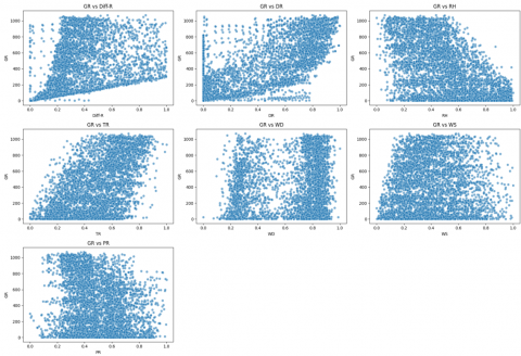
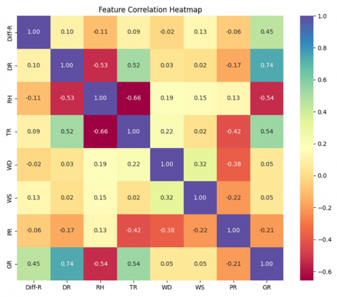
To study the relationships between input features and the target variable, a set of experiments was conducted. Figure 1 shows a series of scatter plots visualizing the relationship between the target variable, GR, and the different features. Each subplot focuses on the correlation between GR and one of the meteorological features. It is clearly observed that there is a strong positive correlation between GR and both DR and TR. This means these two features are major components of evaluating the amount of GR. For features RH and WS, a negative correlation seems to exist; this clearly indicates that higher values tend to be associated with lower GR, and this is as expected, since increasing the amount of clouds and other atmospheric factors such as wind speed will reduce the amount of GR reaching the earth's surface. These findings are also observed when calculating the correlation coefficients that give numeric measures of the relationship between variables, either positive or negative correlation. The heatmap presented in Figure 2 shows that DR has the highest positive correlation coefficient (0.74), and RH has the lowest among the others with -0.54. Other features have either low or moderate correlation with GR.
Figure 1. Pairwise feature relationships: Visualizing correlations between features
Figure 2. Heatmap visualization of features correlation in the dataset
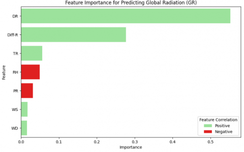
Furthermore, Figure 3 shows the feature importance bar chart, which visually ranks the input features based on their importance in predicting GR. As expected, DR has the strongest positive correlation, as it is the most important feature affecting the amount of GR, and RH is the second most important feature, but with a negative correlation. This means that higher values of RH tend to be associated with lower GR values. The other features (Diff-R, TR, WD, WS, PR) have low to moderate importance ranking in predicting GR, which is also aligned with the previous observations from Figures 1 and 2.
Figure 3. Feature importance analysis for predicting solar irradiance
3.2 Data preprocessing
To prepare the dataset for ML models, a set of preprocessing steps was implemented. We first applied linear interpolation as an imputation technique to handle missing values. It is a mathematical equation used to predict missing values within a specific range by analyzing the linear connections between existing data points. It mainly uses a linear interpolation of the missing values along a predetermined axis, where axis 0 corresponds to rows, and the interpolation step goes along the columns. This method is mathematically represented in Eq. (1) [58], given two data points (x1, y2) and (x2, y2).
$y=y_1+\frac{\left(x-x_1\right)\left(y_2-y_1\right)}{\left(x_2-x_1\right)}$ (1)
where, y is the interpolated value at a point x, (x1, y1) and (x2, y2) are the known data points, and x is the position where the interpolation takes place.
The dataset samples were recorded every 10 minutes, which means that there are 6 readings per hour. To simplify the analysis and focus on hourly-based measurements, we applied an aggregation step to group each 6 consecutive samples into a representative one by taking their mean. Afterward, and since the dataset contained samples for 24 hours, we only focus on the time interval where the solar radiation is effective, the interval that extends from sunshine to sunset duration in the region. For the months of January, February, October, November, and December, we considered the sun duration to be from 6:00 AM to 5:30 PM. For March and April, the duration was from 6:00 AM to 6:00 PM, and for May through September, it was from 5:00 AM to 7:00 PM. So, all samples located outside these periods were filtered out, a manual check was done to make sure all filtered samples have a 0 GR. We applied another filtering step to remove any outliers found in the dataset. For this purpose, we used Inter Quartile Range (IQR), it is a statistical method being widely used to detect and remove outliers from a dataset, it calculates Q1 (25th percentile) and Q3 (75th percentile), it then computes IQR=Q3–Q1, and next it determines the lower and upper bounds as follows: LB=Q1–1.5*IQR, UB=Q3+1.5*IQR, the data points located below the lower bound or above the upper bound are considered outliers, and consequently removed from the dataset [61].
For better comparability between models, it is necessary to make sure that all features contribute equally to the analysis by eliminating differences in magnitude. This process is called data normalization or scaling. It retains the relative distribution of values while bringing values of all variables to a common scale. This process is particularly useful when working with datasets that contain features measured in different units or scales, as it limits or prevents input features with larger ranges from dominating the analysis, ensuring that the results and their analysis are not biased to specific models by magnitudes across the dataset or differences in scale. In this study, we used Min-Max scaling, a widely performed data transformation method, which transforms the data to a fixed range of [0, 1] following Eq. (2) [62].
$\mathrm{x}^{\prime}=\frac{\mathrm{x}-\mathrm{x}_{\min }}{\mathrm{x}_{\max }-\mathrm{x}_{\min }}$ (2)
where, x represents the actual value, xmin and xmax is the minimum and maximum value, respectively, and $x^{\prime}$ is the normalized value.
In summary, the raw dataset contained 52,405 samples, of which 148 had null values. These null values were estimated using interpolation. The data was filtered out based on the sun duration in the region (from sunrise to sunset), considering specific intervals for different seasons, and outliers were removed using the IQR statistical method. The dataset was reduced to 26,952 samples. After the aggregation step, in which every six samples were combined, the processed dataset was further reduced to 4,402 samples, which became the final count.
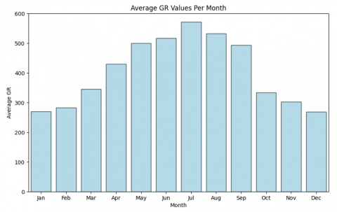
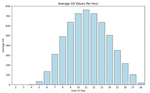
For further visualization of the processed dataset, Figure 4 shows a bar plot of the mean values of GR per month. It is clearly observed that GR values increase from January, reach the peak in the summer months (May, June, July, and August), and then gradually decrease towards December. This tendency suggests a strong seasonal variation in solar radiation. In Winter (Jan, Feb, Dec) there is lower solar radiation due to shorter days (sun duration) and lower solar angles. Spring (Mar, Apr, May), radiation steadily increases as days become longer, and the sun duration, and solar intensity increase. In Summer (Jun, Jul, Aug), the maximum solar radiation occurs, likely due to the longest days and highest solar angles, and in Autumn (Sep, Oct, Nov), solar radiation decreases as days become shorter and solar angles decrease further. To get deeper, Figure 5 represents a histogram of the hourly variation of mean GR (in W/m2) during the day. As it's observed, GR starts extremely low in the early morning hours (around 6:00-7:00 AM), it then increases sharply, reaching the peak around late morning to early afternoon (10 AM to 1 PM). After that, it starts decreasing steadily toward late afternoon (around 4:00-6:00 PM), approaching zero as the day ends.
Figure 4. Monthly variation of average global solar irradiance (W/m2)
Figure 5. Hourly variation of average global solar irradiance (W/m2)
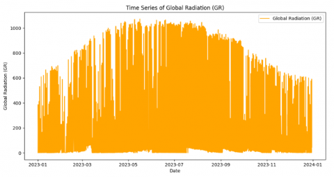
Figure 6 represents GR values (in W/m2) as a timeseries, indicating the intensity of solar radiation received at a given time for 2023. It is shown that GR increases steadily, reaching a peak in the summer months (May to August) due to longer days and higher solar angles, where the highest values of GR are observed around the middle of the year, and decreases gradually as the year progresses toward winter, with shorter days and lower solar angles.
Figure 6. Time series of global solar irradiance (W/m2) for 2023
4.1 Approach
A typical ML approach is employed in this study that begins with data collection, where relevant data is gathered from sensors installed in a meteorological station located in Jerusalem city. Several features relevant to this study were monitored and recorded, such as temperature, humidity, wind speed, wind direction, pressure and solar radiation data. The next step involves data preprocessing, including data cleaning where missing values are handled; data filtering, where outliers and samples recorded outside the sun duration are detected and removed; data aggregation, where data is merged on hourly-based to facilitate the analysis; then data normalization or standardization was applied to ensure that input features are on the same scale, which plays a crucial role in enhancing the performance and convergence of certain ML algorithms. The next step proceeds to the model selection and training phase. Eight ML models, they are RF, SVR, LR, GB, DT, KNN, MLP, and LSTM, are evaluated based on the problem at hand. The models are trained using a subset of the dataset, typically split into training and validation subsets to avoid overfitting. Hyperparameter tuning is also performed, where different configurations of the model’s parameters are evaluated to optimize the overall performance. K-fold cross-validation is also employed to verify that all models generalize well to unseen data. Finally, after training, the models’ performance is evaluated using a set of predefined evaluation metrics such as RMSE, rRMSE, MAE, and R2 [63].
4.2 ML models
This section presents an overview of the eight ML algorithms employed in this study, highlighting their core principles. Each algorithm is selected based on its unique features, ensuring a diverse range of mechanisms to study the solar radiation prediction problem effectively. The selected ML algorithms include both traditional techniques, such as LR, DT, KNN, and SVM, as well as advanced models like RF and GB. Additionally, neural network-based approaches, such as MLP and LSTM, are explored to capture nonlinear relationships between features. By experimenting with this diversity of models, we aim to conduct a comprehensive comparison among them in terms of their performance, providing more insights into the most effective models for predicting global solar irradiance in the region [9, 21, 34, 49]. The subsequent sections give brief overviews of these algorithms.
4.2.1 RF
Rf is a supervised ML algorithm commonly used in regression and classification and regression problems. It is based on ensemble methods that build a set of DT utilizing random subsets of data samples and features. Each DT is trained on a bootstrap sample, where samples are randomly selected with replacement. For regression problems, the target value is estimated by aggregating the outputs of all DTs. For classification, the target class is determined by taking the highest majority votes across all trees [28, 64].
4.2.2 SVR
SVR is a special type of family of ML algorithms called SVM, used mainly for regression tasks. This algorithm aims to predict continuous values by deriving a function that best fits the data samples while maintaining an acceptable margin of tolerance for error rates, i.e., it tries to find an optimal hyperplane that minimizes the error rates within a predefined margin, allowing some error values as long as they are within the determined margin. SVR can handle linear and non-linear problems, but it is particularly useful for the latter one, where the relationship between features behaves in a nonlinear manner, as kernel functions can be used to map data points to a multi-dimensional space [55, 58].
4.2.3 LR
LR is one of the oldest, simplest and widespread ML algorithms being used to model a targeted predicted continuous value. based on one feature (simple LR) or more input features (multiple LR). This scheme assumes a linear relationship between the independent variables (input features) and the dependent one (target). LR aims to find the optimal hyperplane in higher dimensions or the best-fitting line that minimizes the error rates between predicted and actual values [16, 42].
4.2.4 GB
GB is a type of ensemble ML technique for classification and regression that builds strong predictive models by combining multiple results of weak prediction models, typically DT. Unlike bagging methods like RF, which build DT independently, GB constructs trees sequentially, which means that trees are built utilizing the greedy approach with multiple split points to minimize the loss functions, where each new tree tries to tune the error value made by the previous trees. This sequential learning makes GB highly effective for both classification and regression tasks [48, 50]
4.2.5 DT
DT is a widely employed ML algorithm for both regression and classification tasks. They recursively divide data into smaller subsets based on input features’ values, aiming to create a model with a tree-like structure that predicts the value of the target variable. Each internal node might represent a decision based on a specific feature, each branch represents a decision outcome based on values of a feature, each leaf node contains a predicted outcome, and the last level of the tree (leaves) shows the predicted value for that group/class [58, 62].
4.2.6 KNN
KNN is a simple and non-parametric ML algorithm, which excels in both regression and classification tasks. It works by looking at the nearest data points (neighbors), or the k-closest training samples in the feature space, to make predictions using some distance metrics, such as Euclidean distance. KNN is classified as a ‘lazy learner’ because it does not perform any training activities to build an explicit model during the training task. Instead, it makes a copy of the training data and tries to make predictions only when asked to do that; it has to memorize all data points during the prediction task, which could be less efficient in dealing with a high volume of data. The class value is then determined by either taking the majority vote (in classification tasks) or computing the average (in regression tasks) of the K neighbors. This approach enables the algorithm to self-adapt to different patterns and perform predictions based on the local structure of the data [44, 52].
4.2.7 MLP
MLP is a common type of ANNs consisting of multiple, fully connected layers, whether each layer consists of a set of perception elements known as neurons, where all neurons in a layer are connected to all other neurons in a subsequent one, connected in a feedforward manner, and typically use nonlinear activation functions to build models that efficiently deal with complex patterns in data. MLP can be implemented for classification or regression tasks. MLP network typically consists of three layers: input layer, which receives input data and forwards it to the hidden layers, it contains a number of neurons equals to the number of input features; hidden layers, which perform computations and transform the input data using different number of hidden layers; activation function, it is used to apply non-linear transformation to the output of each neuron in the hidden layers, hyperbolic tangent (tanh), Rectified Linear Unit (ReLU), and sigmoid are examples of activation functions. The final output of the network can be a classification label or a regression target, and adjustable parameters for weights and biases that determine the strength of the connection between all neurons in adjacent layers; and a loss function that measures the error difference between the predictions and the actual values [28, 38].
4.2.8 LSTM
LSTM is a specialized type of RNN that is mainly designed to efficiently capture any long-term dependencies in sequential data. Unlike standard Feedforward Neural Networks (FNN), LSTMs include mechanisms for feedback connections, enabling them to leverage any temporal dependency across sequences. They are also specifically designed to address the challenges of the gradient vanishing problem, which is common when training traditional RNNs on long sequences. In its internal structure, LSTM networks use memory cells to regulate the flow of information and are capable of retaining information over an extended set of sequences. Each memory cell consists of three key components: an input gate, a forget gate, and an output gate. The input gate maintains the amount of new input, while the forget gate controls the amount of information to be discarded from the memory cell. Both gates take the current input and the previous hidden state as inputs and produce output values in the interval from 0 and 1, where 0 indicates information to be ignored and 1 indicates information to be retained. The output gate determines how much content of the memory cell contributes to the hidden state [52, 57].
4.3 Evaluation metrics
In order to assess the effectiveness of the models generated using ML algorithms, four commonly used statistical error measurements and analysis techniques in time-series prediction were employed and described in Eqs. (3) to (6) [45, 62]. RMSE provides details regarding how effectively the prediction models perform, where the average magnitude of the error in a sample can be measured by RMSE. Hence, the errors are squared before they are averaged, which leads to an increase in the weight of large errors in the assessment. rRMSE indicates how the residuals are scaled against the actual values and the errors appear relatively. MAE is a measure of the differences between two observations that indicate the same occurrence. The mean absolute values of individual prediction errors for all instances in the test dataset are provided by MAE. R2 evaluates the degree to which actual data points correlate with the statistical assessment of regression prediction accuracy. A model can achieve a high level of prediction accuracy when RMSE, rRMSE and MAE are close to 0 and R2 is close to 1.
It is worth mentioning that the accurate performance analyses that aid in ranking the prediction models can be obtained using any of the statistical approaches described above.
$\operatorname{RMSE}=\left(\frac{1}{\mathrm{n}} \sum_{\mathrm{j}=1}^{\mathrm{n}}\left(\mathrm{y}_{\mathrm{i}}-\widehat{\mathrm{y}}_1\right)^2\right)^{\frac{1}{2}}$ (3)
$\mathrm{rRMSE}=\left(\frac{\frac{1}{\mathrm{n}} \sum_{\mathrm{j}=1}^{\mathrm{n}}\left(\mathrm{y}_{\mathrm{i}}-\widehat{\mathrm{y}}_{\mathrm{l}}\right)^2}{\sum_{\mathrm{j}=1}^{\mathrm{n}}\left(\hat{\mathrm{y}}_{\mathrm{i}}\right)^2}\right)^{\frac{1}{2}}$ (4)
$\mathrm{MAE}=\frac{1}{n} \sum_{j=1}^n\left|y_i-\widehat{y}_l\right|$ (5)
$R^2=1-\frac{\sum_{j=1}^n\left(\mathrm{y}_{\mathrm{i}}-\widehat{\mathrm{y}}_{\mathrm{l}}\right)^2}{\sum_{j=1}^n\left(y_i-\bar{y}\right)^2}$ (6)
where, $y_i$ and $\widehat{y_l}$ represent the actual solar irradiance value and the predicted value of solar irradiance of the sampled data points at the jth moment, respectively. n is the number of sampled moments of the sample, $\bar{y}$ is the average value of the solar irradiance.
In this section, we discuss the performance of the eight ML algorithms used to forecast solar irradiance in Jerusalem. In order to provide an equitable comparison of ML algorithms, they were trained in identical environmental conditions. The algorithms employed in this work (RF, SVR, LR, GB, DT, KNN, MLP, and LSTM) are compared against each other using widely used statistical performance metrics, namely, RMSE, rRMSE, MAE and R2 to maintain the commendable model in predicting solar irradiance at the study site. Furthermore, we employed a grid search method combined with 5-fold cross-validation to optimize the hyperparameters. This method gives more flexibility to systematically explore combinations of parameter values and select the configurations that yield the best performance based on the set of performance metrics. As discussed later in this section, the following hyperparameter ranges were explored for the best-performing model, RF, as an example: number of trees (n_estimators): [50, 100, 150, 200]; maximum tree depth (max_depth): [10, 20, 30, None]; and minimum samples per leaf (min_samples_leaf): [2, 5, 10]. The final selected parameters were: n_estimators =200, max_depth=None, and min_samples_leaf =5.
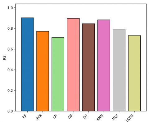
The values of the statistical indicators obtained by the eight models are depicted in Figure 7. R2 values as a function of model performance, as depicted in Figure 7 (a) providing that RF has a value of 0.90, the best accuracy rating out of all the models that were compared. GB, KNN and DT yield values of 0.89, 0.88 and 0.84, respectively. The prediction R2 performance of the other four models (MLP, SVR, LSTM and LR) provide values below 0.8. The value of LR is 0.71, which is the lowest among all compared models.
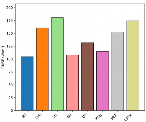
Figure 7 (b) displays the RMSE performance of the models employed. RF is the model that gives the best prediction of the target global solar irradiance variable, delivering predictions with the lowest RMSE value 104.57 W/m2. The GB and KNN returns a value of 107.86 and 114.78, respectively. The other models (DT, SVM, MLP, LSTM and LR) provide relatively high RMSE values of more than 130 W/m2. Meanwhile, LR comes in the last rank and returns a value of 180.49W/m2 with the worst performance.
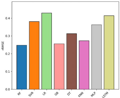
To gain more deeper understanding of how the actual values are scaled over the residuals. The rRMSE values in Figure 7 (c) range from 0.24 for the RF, which is the most efficient model, to 0.43 for the LR, which is the least efficient model. According to the literature [65, 66], RF with such rRMSE value can be classified as a model with good accuracy.
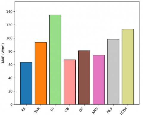
In Figure 7 (d), the MAE comparison with the ML models is shown. It is found that RF presents the best MAE score with associated value of 63.29 W/m2. Meanwhile, GB, KNN, DT, SVM, MLP and LSTM present MAE values ranging from 67.24 to 113.55 W/m2. Once again, the LR performs worst amongst all, with a very high MAE rating of 134.90 W/m2. Furthermore, the model performances of R2, RMSE, rRMSE and MAE provides consistency in ranking the best and worst prediction models; i.e., the higher R2 value matches with the lower RMSE, rRMSE and MAE values. To sum up, the results depicted in Figure 7 show the superiority of RF (R2 = 0.90, RMSE=104.57, rRMSE=0.24 and MAE=63.29) that outperforms the others in predicting solar irradiance in Jerusalem. Among all the models employed, LR (R2=0.71, RMSE=180.49, rRMSE=0.42 and MAE=134.90) presents the worst performance.
(a) R2
(b) RMSE
(c) rRMSE
(d) MAE
Figure 7. Performances of the models (a) R2, (b) RMSE, (c) rRMSE, and (d) MAE
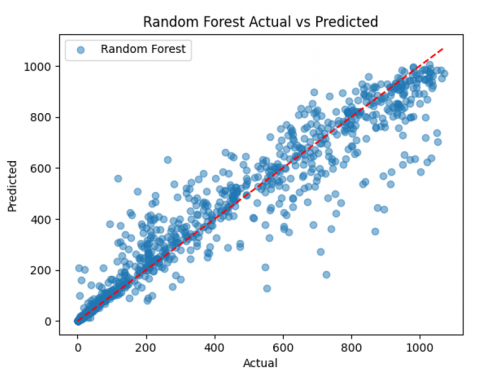
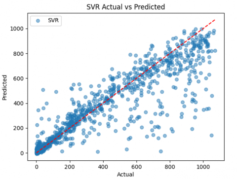
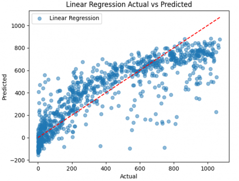
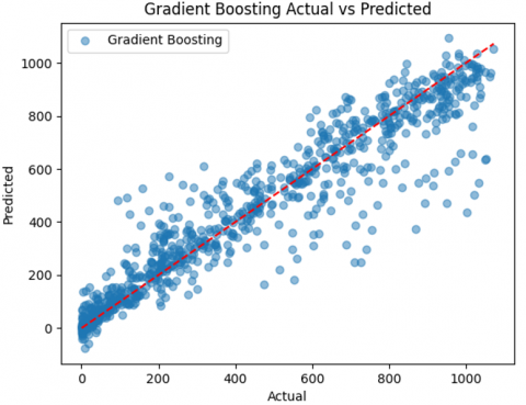
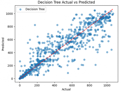
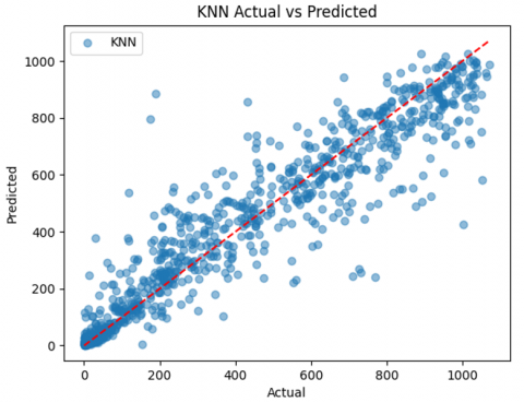
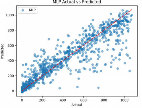
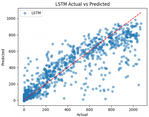
Figure 8 shows comparative scatter plots between actual global solar irradiance versus predicted values of the models employed. As shown in Figure 8 (a), the plotted data points of the best performance model (RF) are generally located near the 1:1 line with very close predictions of lower values and slightly underestimates of higher solar irradiance values. RF provides lower residuals compared to the other models. Very similar results for GB and KNN models (Figures 8 (d) and 8 (f)) with more residuals for both models. Clear underestimation of moderate and higher solar irradiance values provided by SVR (Figure 8 (b)). DT provides good predictions for lower values and overestimates the moderate values as shown in Figure 8 (e), while MPL as presented in Figure 8 (g) overestimates the lower values and underestimates the moderate and higher values. LSTM overestimates the lower and moderate values and underestimates the maximum values as shown in Figure 8 (h). The worst performance prediction values were generated by LR as shown in Figure 8 (c), where LR presents negative predictions for lower solar irradiance values, overestimation of moderate values and highly underestimation of higher values.
(a) RF
(b) SVR
(c) LR
(d) GB
(e) DT
(f) KNN
(g) MLP
(h) LSTM
Figure 8. Scatter plots of predicted versus actual global solar irradiance (W/m2)
Finally, the results presented in Figure 8 are in consistent with those provided by Figure 7. RF is a commendable model in predicting solar irradiance and the results outperform the others, while the results obtained by LR showed lower accuracy; hence, this model should not be used for predicting solar irradiance in the study site.
Table 2 presents a comparative analysis against a selection of studies conducted in various regions, including Turkey, Bangladesh, and others. This comparison focuses on the adjusted R2 metric to provide a more equitable assessment of predictive performance and to ensure consistency across different studies. The results indicate that the proposed model demonstrates competitive performance metrics compared to models from other regions, despite some regional variability.
Table 2. Comparison of the proposed approach with others in terms of the adjusted R2
|
Reference |
Location |
Prediction Models |
Best Model |
R2 |
|
[35] |
Global |
ANN, MEA-ANN, RF, WNN, Empirical |
MEA-ANN |
0.885 |
|
[67] |
Global |
MLR, ANN, Empirical |
ANN |
0.884 |
|
[68] |
Global |
SVR, XGBT, CatBoost, VOA |
VOA |
0.848 |
|
Present work |
Jerusalem, Palestine |
RF, GB, KNN, DT, MLP, SVR, LSTM, LR |
RF |
0.90 |
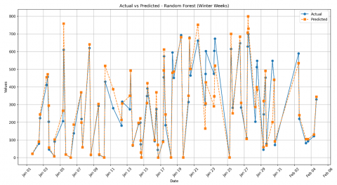
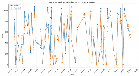
Global solar irradiance pattern in Palestine changes from lower values in winter and higher values in summer. The comparisons of the solar irradiance predictions and real measurement results of the best performance model (RF) that was developed by an ML algorithm for a period of six weeks for both winter and summer in Jerusalem is given in Figure 9. It is seen that RF better estimates the minimum and lower values of global solar irradiance for both winter and summer months. As illustrated in Figure 9 (a) the model presents an overestimation of the maximum values in winter weeks, while it underestimates the maximum global solar irradiance values in summer weeks as depicted in Figure 9 (b).
(a) Winter weeks
(b) Summer weeks
Figure 9. Actual and predicted global solar irradiance (W/m2) comparative performance plot of RF model for six weeks: (a) Winter weeks, (b) Summer weeks
It’s worth mentioning that the summer season in East Jerusalem is characterized by consistently high irradiance levels and prolonged periods of clear skies—conditions that may not be adequately represented in the training data, especially if such periods occur infrequently in other parts of the year. This tendency of RF models to underestimate high irradiance under clear-sky conditions is also supported in the literature. For example, Wan et al. [69] reported a similar underestimation behavior when applying RF to solar radiation estimation in Chongqing, China, particularly during clear and high-radiation periods. This suggests that RF may be limited in extrapolating beyond the range of observed training values or may be affected by averaging effects inherent to ensemble methods.
In this study, we evaluated eight ML models - RF, GB, KNN, DT, MLP, SVR, LSTM, and LR to predict solar irradiance in a study site located in East Jerusalem, Palestine, a city situated within the latitude range of the Mediterranean region. We also analyzed the relative importance of input meteorological features for each model. Among the models tested, RF yielded the best performance, achieving the lowest prediction error (RMSE=104.57, rRMSE=0.24, MAE=63.29) and the highest coefficient of determination (R2=0.90). In contrast, LR exhibited the weakest performance, with RMSE=180.49, rRMSE=0.43, MAE=134.90, and R2=0.71. Future research directions include exploring temporal and spatial generalization by extending the study to additional geographic locations; incorporating additional meteorological and environmental features—such as cloud cover, aerosol optical depth, and atmospheric pressure—where applicable, as these are known to influence solar irradiance levels; investigating real-time deployment scenarios with a focus on lightweight models suitable for solar forecasting on low-power edge devices; and exploring hybrid modeling techniques that combine physical models with data-driven approaches to achieve greater prediction stability and accuracy.
[1] Juaidi, A., Montoya, F.G., Ibrik, I.H., Manzano-Agugliaro, F. (2016). An overview of renewable energy potential in Palestine. Renewable and Sustainable Energy Reviews, 65: 943-960. https://doi.org/10.1016/j.rser.2016.07.052
[2] Alsamamra, H.R., Salah, S., Shoqeir, J.H. (2024). Performance analysis of ARIMA model for wind speed forecasting in Jerusalem, Palestine. Energy Exploration & Exploitation, 42(5): 1727-1746. https://doi.org/10.1177/01445987241248201
[3] West, L.J.S. (2022). Palestinian central bureau of statistics (PCBS). Energy balance of Palestine in physical units, 2022. https://www.pcbs.gov.ps/Portals/_Rainbow/Documents/Energybalance_PH_2022_E.htm.
[4] Khatib, T., Bazyan, A., Assi, H., Malhis, S. (2021). Palestine energy for photovoltaic generation: Current status and what should be next? Sustainability, 13(5): 2996. https://doi.org/10.3390/su13052996
[5] Abboushi, N., Alsamamra, H. (2021). Achievements and barriers of renewable energy in Palestine: Highlighting Oslo Agreement as a barrier for exploiting RE resources. Renewable Energy, 177: 369-386. https://doi.org/10.1016/j.renene.2021.05.114
[6] Gielen, D., Boshell, F., Saygin, D., Bazilian, M.D., et al. (2019). The role of renewable energy in the global energy transformation. Energy Strategy Reviews, 24: 38-50. https://doi.org/10.1016/j.esr.2019.01.006
[7] Nassar, Y.F., Alsadi, S.Y. (2019). Assessment of solar energy potential in Gaza Strip-Palestine. Sustainable Energy Technologies and Assessments, 31: 318-328. https://doi.org/10.1016/j.seta.2018.12.010
[8] Yousefi, H., Hafeznia, H., Yousefi-Sahzabi, A. (2018). Spatial site selection for solar power plants using a GIS-based Boolean-fuzzy logic model: A case study of Markazi Province, Iran. Energies, 11(7): 1648. https://doi.org/10.3390/en11071648
[9] Li, Y.F., Xue, W.L., Wu, T., Wang, H.Z., et al. (2021). Intrusion detection of cyber physical energy system based on multivariate ensemble classification. Energy, 218: 119505. https://doi.org/10.1016/j.energy.2020.119505
[10] Parvin, M., Yousefi, H., Noorollahi, Y. (2023). Techno-economic optimization of a renewable micro grid using multi-objective particle swarm optimization algorithm. Energy Conversion and Management, 277: 116639. https://doi.org/10.1016/j.enconman.2022.116639
[11] Alsamamra, H.R., Salah, S., Shoqeir, J.A., Manasra, A.J. (2022). A comparative study of five numerical methods for the estimation of Weibull parameters for wind energy evaluation at Eastern Jerusalem, Palestine. Energy Reports, 8: 4801-4810. https://doi.org/10.1016/j.egyr.2022.03.180
[12] International Energy Agency (IAE). Renewables 2023: Analysis and forecast to 2028. https://iea.blob.core.windows.net/assets/96d66a8b-d502-476b-ba94-54ffda84cf72/Renewables_2023.pdf.
[13] Jed, M., Ihaddadene, N., Jed, M.E.H., Ihaddadene, R., El Bah, M. (2022). Validation of the accuracy of NASA solar irradiation data for four African regions. International Journal of Sustainable Development & Planning, 17(1): 29-39. https://doi.org/10.18280/ijsdp.170103
[14] Steg, L. (2023). Psychology of climate change. Annual Review of Psychology, 74(1): 391-421. https://doi.org/10.1146/annurev-psych-032720-042905
[15] Eckardt, N.A., Ainsworth, E.A., Bahuguna, R.N., Broadley, M.R., et al. (2023). Climate change challenges, plant science solutions. The Plant Cell, 35(1): 24-66. https://doi.org/10.1093/plcell/koac303
[16] Feng, Z.H., Guo, B., Xu, H., Zhang, L.G., et al. (2021). A new view on the trend of solar radiation in mainland China-based on the optimized empirical model. Theoretical and Applied Climatology, 145(1): 519-532. https://doi.org/10.1007/s00704-021-03643-8
[17] Bouchouicha, K., Hassan, M.A., Bailek, N., Aoun, N. (2019). Estimating the global solar irradiation and optimizing the error estimates under Algerian desert climate. Renewable Energy, 139: 844-858. https://doi.org/10.1016/j.renene.2019.02.071
[18] Ibrik, I.H. (2019). Techno-economic analysis of wind energy resources based on real measurements in West Bank-Palestine. International Journal of Energy Economics and Policy, 9(6): 26-32. https://doi.org/10.32479/ijeep.8067
[19] Alsamamra, H., Ajlouni, E. (2019). A review of solar energy prospects in Palestine. American Journal of Modern Energy, 5(3): 49-62. https://doi.org/10.11648/j.ajme.20190503.11
[20] Palestinian Investment Promotion Agency (PIPA). (2020). Regulation of incentive package contract for the purpose of investment encouragement in the employment of renewable energy technologies No (9) of 2021. https://legal.pipa.ps/files/server/Renewable%20Energy.pdf.
[21] Khosravi, A., Koury, R.N.N., Machado, L., Pabon, J.J.G. (2018). Prediction of hourly solar radiation in Abu Musa Island using machine learning algorithms. Journal of Cleaner Production, 176: 63-75. https://doi.org/10.1016/j.jclepro.2017.12.065
[22] Colak, H.E., Memisoglu, T., Gercek, Y. (2020). Optimal site selection for solar photovoltaic (PV) power plants using GIS and AHP: A case study of Malatya Province, Turkey. Renewable Energy, 149: 565-576. https://doi.org/10.1016/j.renene.2019.12.078
[23] Voyant, C., Notton, G., Kalogirou, S., Nivet, M.L., et al. (2017). Machine learning methods for solar radiation forecasting: A review. Renewable Energy, 105: 569-582. https://doi.org/10.1016/j.renene.2016.12.095
[24] Kumari, P., Toshniwal, D. (2021). Deep learning models for solar irradiance forecasting: A comprehensive review. Journal of Cleaner Production, 318: 128566. https://doi.org/10.1016/j.jclepro.2021.128566
[25] Morf, H. (2021). A validation frame for deterministic solar irradiance forecasts. Renewable Energy, 180: 1210-1221. https://doi.org/10.1016/j.renene.2021.08.032
[26] Demir, V., Citakoglu, H. (2023). Forecasting of solar radiation using different machine learning approaches. Neural Computing and Applications, 35(1): 887-906. https://doi.org/10.1007/s00521-022-07841-x
[27] Ajith, M., Martínez-Ramón, M. (2023). Deep learning algorithms for very short term solar irradiance forecasting: A survey. Renewable and Sustainable Energy Reviews, 182: 113362. https://doi.org/10.1016/j.rser.2023.113362
[28] Liu, J., Huang, X.Q., Li, Q., Chen, Z.Q., et al. (2023). Hourly stepwise forecasting for solar irradiance using integrated hybrid models CNN-LSTM-MLP combined with error correction and VMD. Energy Conversion and Management, 280: 116804. https://doi.org/10.1016/j.enconman.2023.116804
[29] Lara-Benítez, P., Carranza-García, M., Luna-Romera, J.M., Riquelme, J.C. (2023). Short-term solar irradiance forecasting in streaming with deep learning. Neurocomputing, 546: 126312. https://doi.org/10.1016/j.neucom.2023.126312
[30] Lu, Y.B., Wang, L.C., Zhu, C.M., Zou, L., et al. (2023). Predicting surface solar radiation using a hybrid radiative transfer-machine learning model. Renewable and Sustainable Energy Reviews, 173: 113105. https://doi.org/10.1016/j.rser.2022.113105
[31] Ferkous, K., Guermoui, M., Menakh, S., Bellaour, A., Boulmaiz, T. (2024). A novel learning approach for short-term photovoltaic power forecasting—A review and case studies. Engineering Applications of Artificial Intelligence, 133: 108502. https://doi.org/10.1016/j.engappai.2024.108502
[32] Nie, Y.H., Li, X.T., Paletta, Q., Aragon, M., et al. (2024). Open-source sky image datasets for solar forecasting with deep learning: A comprehensive survey. Renewable and Sustainable Energy Reviews, 189: 113977. https://doi.org/10.1016/j.rser.2023.113977
[33] Wang, L.C., Kisi, O., Zounemat‐Kermani, M., Zhu, Z., et al. (2017). Prediction of solar radiation in China using different adaptive neuro‐fuzzy methods and M5 model tree. International Journal of Climatology, 37(3): 1141-1155. https://doi.org/10.1002/joc.4762
[34] Gul, E., Baldinelli, G., Wang, J.W., Bartocci, P., Shamim, T. (2025). Artificial intelligence based forecasting and optimization model for concentrated solar power system with thermal energy storage. Applied Energy, 382: 125210. https://doi.org/10.1016/j.apenergy.2024.125210
[35] Feng, Y., Gong, D.Z., Zhang, Q.W., Jiang, S.Z., et al. (2019). Evaluation of temperature-based machine learning and empirical models for predicting daily global solar radiation. Energy Conversion and Management, 198: 111780. https://doi.org/10.1016/j.enconman.2019.111780
[36] Hou, S., Zhou, Y., Liu, H., Zhu, N. (2017). Wavelet support vector machine algorithm in power analysis attacks. Radioengineering, 26(3): 890-902. https://doi.org/10.13164/re.2017.0890
[37] Yagli, G.M., Yang, D., Gandhi, O., Srinivasan, D. (2020). Can we justify producing univariate machine-learning forecasts with satellite-derived solar irradiance? Applied Energy, 259: 114122. https://doi.org/10.1016/j.apenergy.2019.114122
[38] Sammar, M.J., Saeed, M.A., Mohsin, S.M., Akber, S.M.A., et al. (2024). Illuminating the future: A comprehensive review of AI-based solar irradiance prediction models. IEEE Access, 12: 114394-114415. https://doi.org/10.1109/ACCESS.2024.3402096
[39] Yan, J., Li, K., Bai, E., Yang, Z., Foley, A. (2016). Time series wind power forecasting based on variant gaussian process and TLBO. Neurocomputing, 189: 135-144. https://doi.org/10.1016/j.neucom.2015.12.081
[40] Mutavhatsindi, T., Sigauke, C., Mbuvha, R. (2020). Forecasting hourly global horizontal solar irradiance in South Africa using machine learning models. IEEE Access, 8: 198872-198885. https://doi.org/10.1109/ACCESS.2020.3034690
[41] Li, J.M., Ward, J.K., Tong, J.N., Collins, L., Platt, G. (2016). Machine learning for solar irradiance forecasting of photovoltaic system. Renewable Energy, 90: 542-553. https://doi.org/10.1016/j.renene.2015.12.069
[42] Huang, L.X., Kang, J.F., Wan, M.X., Fang, L., et al. (2021). Solar radiation prediction using different machine learning algorithms and implications for extreme climate events. Frontiers Earth Science, 9: 596860. https://doi.org/10.3389/feart.2021.596860
[43] Qing, X.Y., Niu, Y.G. (2018). Hourly day-ahead solar irradiance prediction using weather forecasts by LSTM. Energy, 148: 461-468. https://doi.org/10.1016/j.energy.2018.01.177
[44] Gairaa, K., Voyant, C., Notton, G., Benkaciali, S., Guermoui, M. (2022). Contribution of ordinal variables to short-term global solar irradiation forecasting for sites with low variabilities. Renewable Energy, 183: 890-902. https://doi.org/10.1016/j.renene.2021.11.028
[45] Kumar, K.R., Kalavathi, M.S. (2018). Artificial intelligence based forecast models for predicting solar power generation. Materials Today: Proceedings, 5(1): 796-802. https://doi.org/10.1016/j.matpr.2017.11.149
[46] Etxegarai, G., López, A., Aginako, N., Rodríguez, F. (2022). An analysis of different deep learning neural networks for intra-hour solar irradiation forecasting to compute solar photovoltaic generators' energy production. Energy for Sustainable Development, 68: 1-17. https://doi.org/10.1016/j.esd.2022.02.002
[47] Meenal, R., Selvakumar, A.I. (2016). Estimation of global solar radiation using sunshine duration and temperature in Chennai. In 2016 International Conference on Emerging Trends in Engineering, Technology and Science (ICETETS), Pudukkottai, India, pp. 1-6. https://doi.org/10.1109/ICETETS.2016.7603089
[48] Alizamir, M., Kim, S., Kisi, O., Zounemat-Kermani, M. (2020). A comparative study of several machine learning based non-linear regression methods in estimating solar radiation: Case studies of the USA and Turkey regions. Energy, 197: 117239. https://doi.org/10.1016/j.energy.2020.117239
[49] Rodríguez, F., Martín, F., Fontán, L., Galarza, A. (2021). Ensemble of machine learning and spatiotemporal parameters to forecast very short-term solar irradiation to compute photovoltaic generators’ output power. Energy, 229: 120647. https://doi.org/10.1016/j.energy.2021.120647
[50] Rajagukguk, R.A., Kamil, R., Lee, H.J. (2021). A deep learning model to forecast solar irradiance using a sky camera. Applied Sciences, 11(11): 5049. https://doi.org/10.3390/app11115049
[51] Muhammad, A., Lee, J.M., Hong, S.W., Lee, S.J., Lee, E.H. (2019). Deep learning application in power system with a case study on solar irradiation forecasting. In 2019 International Conference on Artificial Intelligence in Information and Communication (ICAIIC), Okinawa, Japan, pp. 275-279. https://doi.org/10.1109/ICAIIC.2019.8668969
[52] Ağbulut, Ü., Gürel, A.E., Biçen, Y. (2021). Prediction of daily global solar radiation using different machine learning algorithms: Evaluation and comparison. Renewable and Sustainable Energy Reviews, 135: 110114. https://doi.org/10.1016/j.rser.2020.110114
[53] Mellit, A., Sağlam, S., Kalogirou, S.A. (2013). Artificial neural network-based model for estimating the produced power of a photovoltaic module. Renewable Energy, 60: 71-78. https://doi.org/10.1016/j.renene.2013.04.011
[54] Ssekulima, E.B., Anwar, M.B., Al Hinai, A., El Moursi, M.S. (2016). Wind speed and solar irradiance forecasting techniques for enhanced renewable energy integration with the grid: A review. IET Renewable Power Generation, 10(7): 885-989. https://doi.org/10.1049/iet-rpg.2015.0477
[55] Bamisile, O., Oluwasanmi, A., Obiora, S., Osei-Mensah, E., et al. (2024). Application of deep learning for solar irradiance and solar photovoltaic multi-parameter forecast. Energy Sources, Part A: Recovery, Utilization, and Environmental Effects, 46(1): 13237-13257. https://doi.org/10.1080/15567036.2020.1801903
[56] Chandola, D., Gupta, H., Tikkiwal, V.A., Bohra, M.K. (2020). Multi-step ahead forecasting of global solar radiation for arid zones using deep learning. Procedia Computer Science, 167: 626-635. https://doi.org/10.1016/j.procs.2020.03.329
[57] Solano, E.S., Affonso, C.M. (2023). Solar irradiation forecasting using ensemble voting based on machine learning algorithms. Sustainability, 15(10): 7943. https://doi.org/10.3390/su15107943
[58] Guher, A.B., Tasdemir, S., Yaniktepe, B. (2020). Effective estimation of hourly global solar radiation using machine learning algorithms. International Journal of Photoenergy, 2020(1): 8843620. https://doi.org/10.1155/2020/8843620
[59] Jayalakshmi, N.Y., Shankar, R., Subramaniam, U., Baranilingesan, I., et al. (2021). Novel multi-time scale deep learning algorithm for solar irradiance forecasting. Energies, 14(9): 2404. https://doi.org/10.3390/en14092404
[60] Alam, M.S., Al-Ismail, F.S., Hossain, M.S., Rahman, S.M. (2023). Ensemble machine-learning models for accurate prediction of solar irradiation in Bangladesh. Processes, 11(3): 908. https://doi.org/10.3390/pr11030908
[61] Allal, Z., Noura, H.N., Chahine, K. (2024). Machine learning algorithms for solar irradiance prediction: A recent comparative study. e-Prime-Advances in Electrical Engineering, Electronics and Energy, 7: 100453. https://doi.org/10.1016/j.prime.2024.100453
[62] El-Shahat, D., Tolba, A., Abouhawwash, M., Abdel-Basset, M. (2024). Machine learning and deep learning models based grid search cross validation for short-term solar irradiance forecasting. Journal of Big Data, 11(1): 134. https://doi.org/10.1186/s40537-024-00991-w
[63] Riise, H.N., Nygård, M.M., Aarseth, B.L., Dobler, A., Berge, E. (2024). Benchmark of estimated solar irradiance data at high latitude locations. Solar Energy, 282: 112975. https://doi.org/10.1016/j.solener.2024.112975
[64] Salah, S., Alsamamra, H.R., Shoqeir, J.H. (2022). Exploring wind speed for energy considerations in eastern Jerusalem-Palestine using machine-learning algorithms. Energies, 15(7): 2602. https://doi.org/10.3390/en15072602
[65] Ramírez-Rivera, F.A., Guerrero-Rodríguez, N.F. (2024). Ensemble learning algorithms for solar radiation prediction in Santo Domingo: Measurements and evaluation. Sustainability, 16(18): 8015. https://doi.org/10.3390/su16188015
[66] Despotovic, M., Nedic, V., Despotovic, D., Cvetanovic, S. (2016). Evaluation of empirical models for predicting monthly mean horizontal diffuse solar radiation. Renewable and Sustainable Energy Reviews, 56: 246-260. https://doi.org/10.1016/j.rser.2015.11.058
[67] Antonopoulos, V.Z., Papamichail, D.M., Aschonitis, V.G., Antonopoulos, A.V. (2019). Solar radiation estimation methods using ANN and empirical models. Computers and Electronics in Agriculture, 160: 160-167. https://doi.org/10.1016/j.compag.2019.03.022
[68] Solano, E.S., Dehghanian, P., Affonso, C.M. (2022). Solar radiation forecasting using machine learning and ensemble feature selection. Energies, 15(19): 7049. https://doi.org/10.3390/en15197049
[69] Wan, P.H., He, Y.J., Zheng, C.Y., Wen, J.X., Gu, Z.T. (2025). Estimation of solar diffuse radiation in Chongqing based on random forest. Energies, 18(4): 836. https://doi.org/10.3390/en18040836