Yogita Ajgar*![]() | N. R. Krishnamoorthy
| N. R. Krishnamoorthy![]()
© 2025 The authors. This article is published by IIETA and is licensed under the CC BY 4.0 license (http://creativecommons.org/licenses/by/4.0/).
OPEN ACCESS
Short-term solar irradiation prediction is essential for smooth running of various industries, especially for management of flawless electricity generation and distribution. However, solar datasets are rapid, noisy, and non-linear, making standalone models such as LSTM struggle to extract meaningful patterns for GHI forecasting. The unidirectional nature of LSTM restricts learning to past dependencies only, limiting its ability to forecast sudden irradiance drops. Additionally, vanishing gradient issues in long historical data hinder ability of LSTM to capture complex temporal dependencies, leading to suboptimal forecasting performance. To address these challenges, the proposed model leverages deep learning techniques with a feature-refinement approach. Initially, multiple intrinsic mode functions (IMFs) are extracted from the solar irradiance data, each representing different feature sets. A selection criterion is then applied to retain only the most relevant IMFs, which are integrated to form the input feature set. This refined input is used to train a deep learning network, resulting in day-ahead solar irradiance forecasting model. The performance of the model is evaluated at three distinct locations with varying climatic conditions to test its performance consistency. In the proposed model, reduced error rates are observed, which reflects in lower values of MAPE (2.31%), RMSE (1.55 W/m²), and MAE (1.41 W/m²) as compared to the standalone LSTM model, which records MAPE (3.23%), RMSE (3.21 W/m²), and MAE (1.97 W/m²). Results demonstrate significant improvements over benchmarking method corresponding to more than 90% improvement across all statistical parameters. Also, consistent accuracy across diverse climates highlights robustness of the proposed model which makes it a reliable and versatile solution for practical forecasting applications.
solar irradiation forecasting, CEEMDAN, feature selection, renewable energy, BiLSTM
The evolution in technology enforced raging demand of electricity. To fulfil this demand, most countries still rely on fossil fuels which causes greenhouse effects and environmental pollution [1]. To mitigate these effects, the whole world is exploring renewable energy resources (RER) and started inventing new technological advancements and policies for efficient use, management and alignment of these resources [2].
It is predicted that continuous advancement in RE source based electricity generation would reduce the fossil fuel dependency for electricity generation [3]. Therefore, to boost RE resources-based electricity generation, many initiatives are started. Many RE sources such as geothermal, wind, water and solar are abundantly available on earth. However, owing to specific area wise availability resources are chosen for electricity generation at that site. Amongst all, solar energy is abundant and offers electricity generation with much less negative impact on the nearby environment [4]. In most of the cases RE sources are considered as secondary option for electricity needs, this is because most of the RE sources are not able to produce electricity consistently to fulfil total demand. Moreover, many times it has been consider as more reliable practice to connect RE source-based electricity with gridded network to ensure availability of the electricity in case of failure of RE source-based electricity generation. This makes management of flawless electricity generation and distribution extremely crucial. This highlights need of GHI availability prediction. Thus, for reliable management of RE source-based electricity, forecasting of GHI availability is decisive and essential.
Moreover, a thorough understanding of solar radiation (SR) at that location is vital for both environmental sustainability and economic potential, as evidenced by the influence of SR on agricultural yield, atmospheric circulation, hydrological processes, public health, and ecological services [5]. Similarly, GHI forecasting is crucial in case of managing and commission issues related to meteorology, hydrology, and renewable energy usages [6]. Therefore, from many aspects GHI forecasting ability is important and influences management related to many essential sectors.
India is located in between the equatorial region and tropic of cancer in the northern hemisphere, due to which abundant SR is available almost everywhere. With nearly 2300 to 3200 hours of sunlight in most of the regions per year, India is capable of generating nearly 4-7 kWh/m2 electricity per day using solar radiance [7]. Despite of such huge availability of solar energy, due to its characteristics such as fluctuation, uncertainty and randomness, complete reliance on solar energy for electricity generation needs excellent planning and backup to fulfil total electricity requirement [8]. Herein, GHI forecasting plays crucial role in management of all solar energy related task and this also reduces significant amount of running cost of power systems [9]. Identifying this trail of need for GHI forecasting, present study focuses on development of GHI forecasting method and its implementation.
Researchers have chosen many paths to craft GHI forecasting techniques. These techniques are broadly categorised as physical method, statistical method, machine learning method and hybrid method [10]. The input parameters and forecast horizons commonly defines forecasting performance of any technique. Mostly, the forecasting ability is learned from historic spatial–temporal information which is available in the form of various parameters and this correlation is used as feature defining contributor while improving the accuracy [11]. In the view of this understanding, present work focuses on framing the machine learning technique of GHI forecasting for Indian region. However, to decide strategy and implementation planning of forecasting technique, previous literature is reviewed, and most relevant information is presented as follows.
1.1 Related work
Technological advancements boosted use of machine learning approaches in the field of solar irradiance forecasting which can be tuned for giving more accurate forecast. The machine learning techniques shows capacity of self-learning, with this approach the relation with historic events is analysed and a pattern is learned which is used to forecast future events. The GHI forecasting is attempted using Elman neural network (ELMAN) [12], artificial neural network (ANN) [13], and support vector machine (SVM) [14] as standalone models. Similarly, many deep learning approaches are also tested for GHI forecasting. A group of researchers reviewed performance of recurrent neural network (RNN), long short term memory (LSTM), gated recurrent unit (GRU), and deep neural network (DNN) models for GHI forecasting [15-18]. This study revealed the superior performance of LSTM over other techniques in terms of RMSE. However, since the historic GHI data and other weather parameters are very uncertain and nonlinear, forecasting ability using machine learning models reached at local minima and limited accuracy is being delivered [8]. This prompted researchers to choose approaches wherein multiple techniques are combinedly used to overcome different issues and a collaborative approach can be formed for better accuracy.
Some research groups designed combined approaches in which two networks are fused. In one such approach CNN and LSTM are fused; wherein geographical data is analysed using CNN and LSTM and historic properties of that data are learned [19]. Whereas, the combined CNN-LSTM approach is used for GHI forecasting in Indian regions also [20]. In this approach temporal features are derived from time-series solar irradiance data using LSTM and spatial features are derived from the correlation matrix of several meteorological variables available at that location and neighbouring locations. This approach shows 37%–45% higher forecast skill score over many standalone methods. To mitigate the overfitting issue, a hybrid model is formed using LSTM and gradient boost algorithm, which is when compared with naive predictor and SVM model shows superior performance in terms of RMSE [21]. Many researchers have tested and shown that LSTM shows better performance over other traditional ML or DL models. Therefore, various forms of LSTM are investigated for their potential application in GHI forecasting. A group of researchers compared the forecasting performance of LSTM and BiLSTM for hourly solar radiation forecasting and found that BiLSTM shows better performance than LR, LSTM and SVR with 98.44 W/m2 RMSE, 71.49 W/m MAE [22]. In another attempt, BiLSTM is used in conjunction with CNN and superior performance than CNN-LSTM, GRU-LSTM, LSTM and GRU is demonstrated [23].
Another aspect of the data related to solar irradiance or weather parameters is random fluctuations of readings and time series shows different trends and cycles (depending on season and local geographic conditions) which makes it difficult to learn by simplistic machine learning and deep learning models. This affects the accuracy of prediction ability of forecasting models. To tackle these issues, various data decomposition techniques are employed in conjunction with DL methods. These signal processing techniques clean-up, decompose and align the input vector in accordance with specified guidelines prior to feed to the predictor. Some signal processing techniques such as Wavelet transform (WT) [24], SOM, normalization, Kalman filter, Fourier’s transform (FFT), empirical mode decompositions (EMD) [25], EEMD, CEEMDAN [21], variational mode decomposition (VMD) [26] are used in crafting of forecasting techniques. A research group used EMD for input data decomposition and used as an input for training Auto Regression (AR) method and ANN models for GHI forecasting, resulted in enhanced accuracy than that of the AR and ANN models alone [12]. Similarly, EEMD technique is used in conjunction with Self Organizing Map-Back Propagation (SOM-BP) network and the aggregated output is obtained. In the similar way, few research groups utilized WT to decompose input dataset and used it in conjunction with SVM and ANN model [14, 27]. Following the similar path many forecasting models are proposed to forecast GHI for Indian regions.
A group of researchers used a dataset of single location which is decomposed using WT and then used to train LSTM, BiLSTM and GRU. It is demonstrated that learning ability of LSTM and GRU improves after the use of data decomposition technique and accuracy for 24-h ahead GHI forecasting increases [28]. The similar group demonstrated use of full wavelet packet decomposition (FWPD) method for single location input data decomposition and used it to train BiLSTM for 24-hr ahead GHI forecasting [24, 29]. A group of researchers used a dataset of single location which is decomposed using CEEMDAN and then used to train LSTM and GRU. It is demonstrated that learning ability of LSTM and GRU improves after the use of data decomposition technique [30].
On the parallel lines, a group of researchers used a dataset of single location and EEMD is used for input data decomposition thereafter the most prospective sets of features are selected using the Genetic Algorithm (GA) which is then used for training LSTM [31]. Similar group also presented the method wherein CEEMDAN is used in conjunction with GA and BiLSTM for the same single location [32]. For both the studies it is demonstrated that selecting the most prospective sets of features using GA shows improved forecasting accuracy. A research group formulated eleven different models for two different locations using various data decomposition techniques such as VMD, WT, EMD, EEMD, CEEMDAN and WPD prior feeding input to Feedforward neural network (FFNN), LSTM, GRU and BiLSTM. Thereafter, the autocorrelation function (ACF) and partial autocorrelation function (PACF) is employed to select best combination of time lagged data. The results stated that the performance of the WPD based BiLSTM model surpasses all standalone and hybrid models. On similar lines, a group of researchers pre-processed input dataset of four different locations using EMD, EEMD and SEEMDAN and Pearson’s Correlation Coefficient (PCC) is used to find highest correlation coefficient values which are combined to form a single input for Adaptive Neuro Fuzzy Inference System (ANFIS) to form GHI forecasting system [33]. This method demonstrated accuracy with less than 2% MAPE for season wise short-term solar irradiance forecasting. In the view of discussion, present study utilizes CEEMDAN method to pre-process input data. Further, the PCC method is employed for selecting the prospective features. The selected input features are then used to develop forecasting model using BiLSTM. Three locations with different climatic conditions are considered for model testing. The main contribution and highlights of the present work are as follows:
2.1 Equations
The data decomposition technique known as Complete ensemble empirical mode decomposition with adaptive noise (CEEMDAN) is developed and derived through several stages such as EMD, EEMD, and CEEMD. The basic idea of EMD is decomposition of non-linear and non-stationary data. The data decomposition is sorting the dataset with different frequencies and scales in several IMFs and residuals. However, in this technique similar elements are mapped in different IMFs. To overcome mode mixing issue EEMD is proposed, but after IMF reconstruction, it is prone to addition of Gaussian white noise leading to incorporation of error. To resolve these issues CEEMDAN is proposed [34, 35]. The CEEMDAN method sorts the dataset into different IMFs along with one residue. Following steps are carried out to generate IMFs using CEEMDAN technique.
As a first step, Gaussian noise $W_n(t)$ and noise standard error $(\varepsilon)$ are added to original data sequence, and the process can be represented mathematically as
$k_n(t)=k(t)+\varepsilon_o W_n(t)$ (1)
where, $n$ changes from 1 to m with the difference of 1.
In the second step, average of all decomposed component is considered to calculate IMF
$I M F_1(t)=\frac{1}{x} \sum_{i=1}^x I M F_1^i(t)$ (2)
To calculate residue following relation is used
$r_1(t)=k(t)-I M F_1(t)$ (3)
In the third step, EMD is used to decompose ${{r}_{1}}\left( t \right)+~{{\varepsilon }_{1}}EM{{D}_{1}}{{w}_{n}}\left( t \right)$ and second IMF and residue are obtained using following Eqs. (4) and (5).
$I M F_2(t)=\frac{1}{x} \sum_{n=1}^x E M D_1\left(r_1(t)+\varepsilon_1 E M D_1\left(w_n(t)\right)\right.$ (4)
$r_2(t)=r_1(t)-I M F_2(t)$ (5)
Following the similar trend, rest of the IMFs and residues are computed up to the SD value in the following Eq. (6) reaches to 0.2
$\underset{q=0}{\overset{Q}{\mathop \sum }}\,\frac{{{\left| {{r}_{x-1}}\left( t \right)-{{r}_{x}}\left( t \right) \right|}^{2}}}{r_{x-1}^{2}\left( t \right)}\le S{{D}_{x}}$ (6)
where, $Q$ is to keep accountability of the length of sequence and the sequence $K(t)$ after $x^{\text {th }}$ decomposition is denoted as ${{r}_{x}}\left( t \right)$.
At last, following Eq. (7) is used to reconstruct the signal $K(t)$ considering final residual function $R\left( t \right)$.
$y\left( t \right)=\underset{i=1}{\overset{T}{\mathop \sum }}\,IM{{F}_{i}}\left( t \right)+R\left( t \right)$ (7)
2.2 Pearson's Correlation Coefficient (PCC)
In previous few attempts [36, 37], all decomposed components are used as input to train forecasting neural network architecture. However, later studies included the IMF selection strategy with which only feature set with prospective higher correlation with GHI forecasting is considered as input for training forecasting neural network architecture [31-33]. The PCC is being used to evaluate the relationship between two continuous variables. Both strength of the relationship and its dependency direction are evaluated using PCC. The method takes into account reliance on covariance and therefore can be used effectively for assessing associations of the variables.
This type of data sorting is important when dataset is very complex such as weather parameters, solar irradiance and many other time series datasets. In the present case, solar GHI time series dataset shows different trends, random fluctuations and cycles. This makes forecasting modelling difficult and vast scope for random predictions is caused due to use of such dataset. To solve this issue, prospective selection of feature dataset is beneficial. Present work utilizes PCC for identification of prospective feature dataset. In the present work, PCC is calculated for a set of objective variables (X, Y) and defined as follows.
$\mathrm{P}_{(X, Y)}=\frac{\sum\left(X_i-\bar{X}\right)\left(Y_i-\bar{Y}\right)}{\sqrt{\sum\left(X_i-\bar{X}\right)^2 \sum\left(Y_i-\bar{Y}\right)^2}}$ (8)
In this Eq. (8), $\mathrm{P}_{(X, Y)}$ is Pearsons correlation coefficient, which is calculated using Values of x and y variables denoted as $X_i$ and $Y_i$ respectively in sample set. Similarly, mean of the values of the x and y variable are denoted as $\bar{X}$ and $\bar{Y}$ of a sample set.
2.3 LSTM
Figure 1. Fundamental architecture of LSTM
The Recurrent Neural Network (RNN) is structured in 1982 to process the data with certain sequence. In case of RNN, its output is again connected to input via feedback, serving as a kind of dynamic memory [36]. This network worked well for short-term forecasting, but unstable results are obtained in case of long-term forecasting. It is then realized that, the vast gradient, or abruptly significant changes in training weights causing this instability [38]. By permitting memory cells in the hidden layer(s), the LSTM network offered a solution to the vast gradient problem. The memory cells are included in layer to selectively discard the information from dataset or retain the information in dataset. Figure 1 depicts the fundamental architecture of LSTM. LSTM contains memory cells which are constituted using input gate (it), output gate (ot) and forget gate (ft), with the help of which information can be accepted or rejected. To operate forward movement function, the output value ht-1 from previous cell ‘Ct-1’ is also considered. In the present time ‘t’, three input for LSTM are considered, which are output of previous cell ‘$h_{t-1}$’, bias ($b$) and $x_t$ use here parameter (P) [38]. Similarly, weight vectors are signified as “W”. For considering the next parameter, the network needs to forget the previous parameter, therefore following step is considered.
$f_t=\sigma\left(W_f .\left[h_{t-1}, x_t\right]+b_f\right)$ (9)
To decide next information to be stored in cell is decided using two operations. In the first operation a next value is decided via a sigmoid layer also denoted as input gate layer using following Eq. (10).
$i_t=\sigma\left(W_i \cdot\left[h_{t-1}, x_t\right]+b_i\right)$ (10)
After which, in second operation, the vector of next value is created using tanh layer.
$\tilde{C}_t=\tanh \left(W_C .\left[h_{t-1}, x_t\right]+b_C\right)$ (11)
Finally, the new cell state is updated using following Eq. (12).
$C_t=f_t * C_{t-1}+i_t * \tilde{C}_t$ (12)
Now, to decide output, first using sigmoid layer, a part of cell is selected for output.
$o_t=\sigma\left(W_o \cdot\left[h_{t-1}, x_t\right]+b_o\right)$ (13)
At last, the cell state is put through tanh which decide the value between -1 to 1 and multiplication of it with output of output gate produces selective output which needed to be carry forward for next step.
$h_t=o_t * \tanh \left(C_t\right)$ (14)
2.4 BiLSTM
In case of BiLSTM, both backward and forward movement functioning is possible. The hidden characteristics and pattern of the data can be revealed while processing is carried out in backward direction [39]. The identification of such patterns is absent in case of LSTM which proceeds only in forward direction, therefore choosing BiLSTM becomes beneficial in case of long historic weather-related database wherein many such hidden patterns can be identified if processed properly. Figure 2 depicts the fundamental architecture of BiLSTM [22].
Figure 2. Fundamental architecture of BiLSTM
For updating the network, the backward hidden layer ‘$H L_b$, output sequence ‘$x_0(t)$, and forward hidden layer ‘$H L_f$’ are considered. With this initiation, the network of BiLSTM updates iteratively in backward and forward direction. Output for forward pass forward ($H L_f$), backward pass backward ($H L_b$) and output parameter from that layer ($x_0(t)$) is calculated using following Eqs. (15) to (17).
$H{{L}_{f}}$=$\sigma \left( {{W}_{1}}~{{x}_{t}}+{{W}_{2}}~H{{L}_{f-1}}+{{b}_{H{{L}_{f}}}} \right)$ (15)
$H{{L}_{b}}$=$\sigma \left( {{W}_{3}}~{{x}_{t}}+~{{W}_{5}}~H{{L}_{b-1}}+{{b}_{H{{L}_{b}}}} \right)$ (16)
${{x}_{0}}$=${{W}_{4}}~H{{L}_{f}}+{{W}_{6}}~x+{{b}_{{{x}_{0}}}}$ (17)
where, weights coefficients are denoted as W and the biases are signified as ‘$b_{H L_f}$’, ‘$b_{H L_b}$’ and ‘$b_{x_0}$’.
2.5 Performance assessment
The GHI forecasting models are assessed using different matrices such as MAPE, RMSE and MAE. These matrices are symbolic and persuasive, which makes them reliable for testing the forecasting ability of the present developed models. The results shown by these matrices enhances the acceptability of these models for real world application. The following Eqs. (18) to (20) are used to calculate respective type of error, where $y_i$ is the result predicted by the model; ŷi is the actual test sample value; and n is the total number of test samples.
$M A E_{(y, \hat{y})}=\frac{1}{n} \sum_{i=1}^n\left|y_i-\hat{y}_i\right|$ (18)
$M A P E_{(y, \hat{y})}=\frac{1}{n} \sum_{i=1}^n\left|\frac{y_i-\hat{y}_i}{y_i}\right|$ (19)
$R M S E_{(y, \hat{y})}=\sqrt{\frac{1}{n} \sum_{i=1}^n\left(y_i-\hat{y}_i\right)}$ (20)
2.6 Network architecture and workflow for GHI forecasting
Combining the aspects of CEEMDAN-PCC-BILSTM, a model is developed to forecast 1-day ahead GHI for three different locations. Overall workflow of the CEEMDAN-PCC-BILSTM is as follows.
3.1 Dataset description
In this study three locations from India located in Maharashtra state, are considered. These locations are chosen by considering Koppen-Geiger stated different climatic conditions. The locations are Nagpur, Jalgaon and Pune. Nagpur with Lat./Long. 21.146633°/79.088860° shows tropical wet and dry climate (Köppen Aw). Jalgaon with Lat./Long. 21.004194° /75.563942° shows hot semi-arid climate (Köppen BSh). Pune with Lat./Long. 18.516726°/73.856255° shows a tropical wet and dry (Köppen Aw) climate, closely bordering upon a hot semi-arid climate (Köppen BSh).
The GHI data for these three locations is accessed from NSRDB or NIWE national data portal. The GHI data is collected hourly with 30-minute gap over the period of June 2016- May 2019. The input data is important and impacts the training of forecasting model. The GHI data collected is non-linear and random this may cause flaws in training forecasting model. Similarly, reading with weak pyranometer reaction may introduce incomplete and negative data recording in the dataset [19]. These entries are cleared before further processing. Also, since solar irradiation is absent at night, the GHI data points of night hours are discarded. This is because large blocks of zero values may bias the model by overfitting toward predicting zeros, thereby reducing sensitivity to variations during the day when forecasting is required. Moreover, since the focus of the present models is day-ahead GHI forecasting for power generation application, the exclusion of night-time data does not compromise model generalizability to operational scenario. However, it is acknowledged that excluding night-time data may bias the model toward daylight conditions, making it unsuitable for applications requiring a full 24-hour solar profile (e.g., thermal storage or nocturnal cooling). In such cases, training with night-time zeros can ensure continuity. However, for daytime GHI forecasting aimed at solar power generation and grid integration, exclusion improves efficiency, reduces noise, and enhances accuracy without affecting practical generalizability.
Similarly, GHI data points collected just before the sunset and just after sunrise are introduced with cosine error of instruments and therefore necessary to be removed. Data points in both these condition shows solar zenith angle greater than 80° and therefore these data points can be removed easily [40]. After this, the dataset is categorized in four seasons as monsoon (June–September), autumn (October–November), winter (December-February) and summer (March–May). Further, to enhance input data set quality, data is converted into stationary form by considering normalized value of data. The normalize value is calculated using following Eq. (21) [41].
${{X}_{norm}}=\frac{X-{{X}_{min}}}{{{X}_{max}}-{{X}_{min}}}$ (21)
where, standardized value is denoted as ${{X}_{norm}}$, X is the original value from dataset, and minimum and maximum values from dataset are denoted as ${{X}_{min}}$ and ${{X}_{max}}$ respectively.
3.2 Hyperparameter selection approach
After the data processing, choice of hyperparameters for training forecasting models plays crucial role and influence the prediction accuracy. Therefore, the present work considered following approach. At the beginning the dataset is divided into two sections for training and testing. By accounting the previously reported approaches [42-44] nearly 80% dataset is assigned for training from where prospective IMF functions are selected using PCC and used for training the forecasting model. Similarly, 20% dataset is considered for testing and validating the outcomes from forecasting model. This is followed for each location separately, wherein, data of first two years is used for training and third year data is used for testing.
3.3 Reconstruction of input for training
As described earlier, dataset of first two years is used for training the forecasting model for each three locations separately. However, before using this dataset for training, several processing steps are followed to select prospective input for enhancing the forecasting ability of the model. First pre-processing step is cleaning of the dataset after which, two years GHI time series data is segmented into four seasons viz. Monsoon (June–September), autumn (October–November), winter (December-February) and summer (March–May). On this data, CEEMDAN decomposition technique is applied to generate 10 IMF and 1 residue for each season. Figure 3 shows IMFs and residue plots for autumn season for Jalgaon city. To select prospective IMFs with prospective feature sets, PCC is used.
Table 1 shows the PCC values for the decomposed IMFs obtained using CEEMDAN. For every location, season wise IMFs and corresponding Residual are obtained using CEEMDAN and compared amongst each other to find highest correlation coefficient values. To avoid overfitting the model, for each location, all season wise IMFs showing PCC 0.5 and above are combined with residue to form a single input. Finally, using this single input, models are trained to forecast one day ahead GHI, for three different locations.
Figure 3. Decomposition results of GHI of autumn season for the Jalgaon city obtained using CEEMDAN
Table 1. Details of PCC with corresponding IMFs using CEEMDAN for different seasons for different cities
|
Location |
Site |
IMF1 |
IMF2 |
IMF3 |
IMF4 |
IMF5 |
IMF6 |
IMF7 |
IMF8 |
IMF9 |
IMF10 |
Residual |
|
Jalgaon |
Autumn |
0.31733 |
0.53508 |
0.61992 |
0.5582 |
0.61172 |
0.16971 |
0.06092 |
0.01821 |
0.01118 |
0.00912 |
0.01593 |
|
Monsoon |
0.26878 |
0.36494 |
0.48948 |
0.51081 |
0.72306 |
0.45989 |
0.14267 |
0.08957 |
0.05258 |
0.04123 |
0.08116 |
|
|
Summer |
0.30523 |
0.52984 |
0.59883 |
0.54713 |
0.63149 |
0.14236 |
0.05891 |
0.03691 |
0.02608 |
0.02256 |
0.05103 |
|
|
Winter |
0.2992 |
0.50198 |
0.58981 |
0.56564 |
0.66037 |
0.46905 |
0.04535 |
0.0378 |
0.02567 |
0.02199 |
0.02451 |
|
|
Pune |
Autumn |
0.32958 |
0.56942 |
0.61502 |
0.55465 |
0.59339 |
0.17858 |
0.04598 |
0.00951 |
0.01285 |
0.01016 |
0.02401 |
|
Monsoon |
0.27595 |
0.4031 |
0.51309 |
0.51598 |
0.71025 |
0.40105 |
0.12636 |
0.08114 |
0.06308 |
0.06165 |
0.10794 |
|
|
Summer |
0.31933 |
0.39148 |
0.62088 |
0.56382 |
0.59801 |
0.12595 |
0.0693 |
0.04927 |
0.03018 |
0.02765 |
0.02587 |
|
|
Winter |
0.32099 |
0.54192 |
0.57933 |
0.56093 |
0.65046 |
0.49023 |
0.12019 |
0.06104 |
0.0589 |
0.03965 |
0.04603 |
|
|
Nagpur |
Autumn |
0.30181 |
0.50119 |
0.60167 |
0.57094 |
0.63992 |
0.36083 |
0.07558 |
0.03299 |
0.00114 |
0.01012 |
0.06693 |
|
Monsoon |
0.24983 |
0.30595 |
0.42948 |
0.46206 |
0.72933 |
0.61096 |
0.15046 |
0.11026 |
0.08603 |
0.07925 |
0.09599 |
|
|
Summer |
0.26704 |
0.51401 |
0.59093 |
0.54025 |
0.62084 |
0.21012 |
0.08032 |
0.04594 |
0.0451 |
0.03925 |
0.05503 |
|
|
Winter |
0.27025 |
0.51998 |
0.57503 |
0.57028 |
0.68514 |
0.51095 |
0.05609 |
0.05505 |
0.03392 |
0.03156 |
0.05045 |
3.4 Training and testing
The models in the present work are trained to forecast 24-h ahead solar GHI, specifically to consider month wise data separately. This is also helpful in fine tuning the model from a season wise perspective. To evaluate the credibility of each step considered in the framework of this model, we trained standalone BiLSTM, then the BiLSTM coupled with CEEMDAN and finally CEEMDAN-PCC-BiLSTM coupled together which sorts most correlated input for model training. This is to investigate that fine tuning of hyperparameters along with initialization of input holds much importance for achieving better accuracy. Even though there are no specific rules for setting hyperparameters we have chosen the following hyperparameters for training present model and kept it constant throughout experimentation. In the present study Adam Optimizer is used. Initially, reference values for the parameters were taken from [32, 24]. Based on preliminary experimental results, the parameters were then finalized as 250 Epoch, 0.0001 learning rate, 200 hidden units, 0.01 gradient units. Since the model training considered month wise (season wise) training, the testing is also carried out on seasonal basis, wherein prediction accuracy for four seasons viz., autumn, monsoon, summer and winter are tested separately. The real solar GHI is predicted by using normalized predicted sequence and actual values are calculated using following Eq. (22) which reveal the relation between denormalized value $({{X}_{denorm}})$ and normalized value $\left( {{X}_{norm}} \right)$ , maximum value $({{X}_{max\text{ }\!\!~\!\!\text{ }}})$, minimum value $({{X}_{min}})$.
${{X}_{denorm}}={{X}_{min}}+\text{ }\!\!~\!\!\text{ }\left( {{X}_{max\text{ }\!\!~\!\!\text{ }}}-{{X}_{min}} \right)\times {{X}_{norm}}$ (22)
In this study, CEEMDAN-PCC-BiLSTM are combined to form a framework of the model which is used to forecast 24-h ahead solar irradiance (GHI). Three different locations as Jalgaon, Nagpur and Pune, from India are chosen for this study. To test the proficiency of the model, the performance is compared with other standalone models such as, Gate Recurrent Unit (GRU), Back Propagation Neural Network (BPNN), RNN, LSTM and BiLSTM and similarly with other methods reported in the literature. For experimentation, MATLAB 2019a is chosen and all the models are implemented and analyzed. The deep learning hyper parameters are carefully tunes to forecast this short term GHI which is season wise categorized. For training data of two years is used while testing is conducted using one year data. The evaluation matrices such as MAPE (%), MAE (W/m2) and RMSE (W/m2) are calculated for analyzing prediction accuracy and ease of comparison.
Table 2. Statistical analysis (MAPE (%)) of a day ahead GHI forecasting for location Jalgaon
|
MAPE (%) |
|||||
|
Models |
Summer |
Monsoon |
Autumn |
Winter |
Annual |
|
BPNN |
4.01 |
6.12 |
4.16 |
4.31 |
4.61 |
|
RNN |
3.11 |
5.1 |
4.12 |
3.56 |
3.91 |
|
GRU |
2.71 |
4.9 |
2.89 |
3.66 |
3.56 |
|
LSTM |
2.16 |
4.54 |
2.68 |
3.58 |
3.23 |
|
BiLSTM |
1.85 |
4.21 |
2.21 |
3.39 |
3.16 |
|
CEEMDAN -BiLSTM |
1.69 |
4.02 |
1.98 |
2.51 |
2.65 |
|
Proposed Model |
0.99 |
3.7 |
1.36 |
2.08 |
2.31 |
Table 3. Statistical analysis (RMSE(W/m2)) of a day ahead GHI forecasting for location Jalgaon
|
RMSE(W/m2) |
|||||
|
Models |
Summer |
Monsoon |
Autumn |
Winter |
Annual |
|
BPNN |
2.99 |
5.89 |
3.63 |
3.51 |
4.18 |
|
RNN |
2.56 |
4.98 |
2.89 |
3.47 |
3.59 |
|
GRU |
2.32 |
4.21 |
2.41 |
3.12 |
3.35 |
|
LSTM |
2.01 |
3.86 |
2.35 |
2.78 |
3.21 |
|
BiLSTM |
1.83 |
3.56 |
1.57 |
1.86 |
2.62 |
|
CEEMDAN -BiLSTM |
0.71 |
3.13 |
1.13 |
1.73 |
2.01 |
|
Proposed Model |
0.36 |
2.58 |
0.88 |
1.59 |
1.55 |
For the sake of simplicity and ease in explanation, at first statistical analysis of single location is considered. To analyze proficiency of the framed strategy used to develop final model, step by step analysis is carried out. For this Jalgaon is chosen as the first location and using this data, all the standalone models are trained. Similarly, in case of CEEMDAN-BiLSTM, the model is trained using all the IMFs summarized in Table 1 and further based on PCC values, selected IMF functions are used to train final proposed CEEMDAN-PCC-BiLSTM model.
Table 4. Statistical analysis (MAE (W/m2)) of a day ahead GHI forecasting for location Jalgaon
|
MAE (W/m2) |
|||||
|
Models |
Summer |
Monsoon |
Autumn |
Winter |
Annual |
|
BPNN |
2.41 |
5.41 |
3.21 |
3.61 |
3.91 |
|
RNN |
1.89 |
4.98 |
3.78 |
2.98 |
3.12 |
|
GRU |
1.61 |
3.65 |
2.61 |
2.61 |
2.51 |
|
LSTM |
1.35 |
3.21 |
1.85 |
2.35 |
1.97 |
|
BiLSTM |
1.15 |
3.14 |
1.53 |
1.97 |
1.77 |
|
CEEMDAN -BiLSTM |
0.98 |
2.96 |
1.08 |
1.56 |
1.64 |
|
Proposed Model |
0.73 |
2.86 |
0.45 |
1.18 |
1.41 |
For ease of analysis, only a single location is considered at first and then the viability of the proposed model is extended to other locations. First the data from Jalgaon location is used to train all the models and observed data is tabulated. In Table 2 (MAPE(%)), Table 3 (RMSE(W/m2)), Table 4 (MAE (W/m2)) statistical analysis for all the standalone models such as BPNN, RNN, GRU, LSTM and BiLSTM are tabulated along with CEEMDAN-BiLSTM and proposed model.
It can be observed from Table 2 that the MAPE for standalone models resulted in the following range as BPNN 4.01-6.12%, RNN 3.11-5.1%, GRU 2.71-4.9%, LSTM 2.16-4.54% and BiLSTM 1.85- 4.21%. In a similar way, RMSE for standalone model range as BPNN 2.99-5.89 W/m2, RNN 2.56-4.98 W/m2, GRU 2.32-4.21 W/m2, LSTM 2.01-3.86 W/m2 and BiLSTM 1.69-4.02 W/m2. Also, the MAE values range for standalone models as BPNN 2.41-5.41 W/m2, RNN 1.89-4.98 W/m2, GRU 1.61-3.65 W/m2, LSTM 1.35-3.21 W/m2 and BiLSTM 1.12-3.1 W/m2. A similar trend has been observed when data from other locations is used to train all these models. All the statistical data revealed that BiLSTM outperforms over all the other standalone models which agrees with previously published reports [22, 23]. This also recites the fact that BiLSTM models are suitable for the use of forecasting models wherein timeseries data is used.
It is important to note here that since standalone deep learning models such as BPNN, RNN and GRU fine adjustment of learning parameters is not considered it limits the forecasting ability of these models. As compared to these models, LSTM performs better, however, unidirectional training and information processing enhances training time and limits performance. Therefore, to overcome these limitations, the proposed model uses BiLSTM as its foundational base.
To validate this observation further, all the above experimentation is repeated using the data of other two locations viz., Nagpur and Pune. To observe other meaningful trends, the graphical representation of the MAPE (%), MAE (W/m2) and RMSE (W/m2) for standalone models such as BPNN, RNN, GRU, LSTM and BiLSTM along with CEEMDAN-BiLSTM and proposed models are also presented.
Another important aspect of the proposed model is global horizontal irradiance input data is decomposed using CEEMDAN preprocessing technique, which generate ten IMFs and one residue. When all IMFs are used to train the BiLSTM network, improvement in forecasting accuracy is evident. This is cited from reduced forecasting errors in CEEMDAN-BiLSTM models for all the cities (Tables 2-4 and Figures 4-6). The CEEMDAN-BiLSTM model outperforms the standalone BiLSTM model since CEEMDAN removes mode mixing constraints and holds the input time series data to improve the quality of training data.
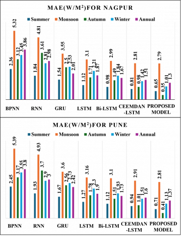
Figure 4. The statistical analysis of the proposed model in terms of MAPE for Nagpur and Pune location
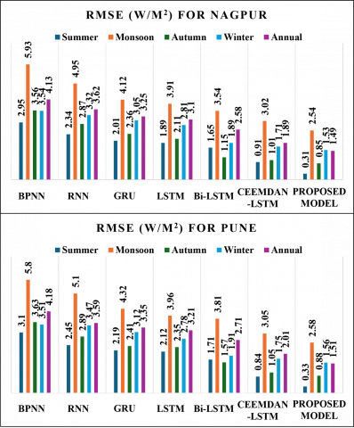
Figure 5. The statistical analysis of the proposed model in terms of RMSE for Nagpur and Pune location
Figure 6. The statistical analysis of the proposed model in terms MAE for Nagpur and Pune location
However, literature shows that considering only most relevant data for training deep neural network can improve its performance. Therefore, in the present case, PCC is calculated for each IMF generated and only the IMF with 0.5 and above PCC values are combined to form an input. Using this input, BiLSTM network is trained which is the concept of proposed model and denoted as CEEMDAN-PCC-BiLSTM model. It can be observed from Tables 2-4. that this model shows annual MAPE as 2.32%, RMSE as 1.55 W/m2 and MAE as 1.41 W/m2 respectively for Jalgaon, which demonstrates outperformance of the proposed models as compared to other models. Similarly, Figures 4-6 demonstrated that for Nagpur location with 2.2% MAPE, 1.49 W/m2 RMSE and 1.3 W/m2 MAE, proposed model outperforms other models. On the similar line, for Pune location with 2.27% MAPE, 1.51 W/m2 RMSE and 1.37 W/m2 MAE, proposed model outperforms other models. These results showcase the forecasting performance credibility of the proposed model for all the locations. Further detailed analysis suggests that use of CEEMDAN and PCC to process the input enhances learning outcomes specially for summer and autumn as compared to winter and monsoon. This may be because summer and autumn shows persistent clear environmental circumstances which supports model to correlate more significantly between forecasted and measured GHI at that time. On the other hand, presence of clouds in rainy days and other fast changing environmental parameter in monsoon and winter increases correlation difficulties between forecasted and measured GHI, leading to increased errors in GHI forecasting.
Finally, performance of the proposed model is compared with previously reported techniques which use other neural network-based learning strategies for GHI forecasting. We also compared the performance with day-ahead persistence model which is considred as standard benchmarking reference in the field of irradiance forecasting. We included the statistical analysis related to the persistence model for all the three locations and compared the performance of proposed model. Table 5 presents the comparative performance of the proposed model with other models in terms of MAPE, RMSE and MAE.
Table 5. Performance comparison of the proposed model with other reported models
|
Time Horizon |
Ref |
Location |
Model |
MAPE (%) |
RMSE (W/m2) |
MAE (W/m2) |
|
24 h 24-h |
- [45] |
Jalgaon, India Nagpur, India Pune, India Qingdao, China |
Persistence Model DFT + PCA + Elman/BPNN |
10.2 10.8 11.3 _ |
145 138 156 127.3 |
33.8 32.5 34.2 _ |
|
1-h |
[20] |
SanDiego, USA |
LSTM–CNN |
_ |
42.89 |
27.38 |
|
1-h |
[18] |
New Delhi, India |
XGBF-DNN |
51.35 |
||
|
1-h |
[22] |
US |
BiLSTM |
_ |
98.44 |
_ |
|
24-h |
[24] |
Ahmadabad, India |
WT + BiLSTM |
6.48 |
45.61 |
_ |
|
24 h |
Proposed model |
Jalgaon, India |
CEEMDAN-PCC-BiLSTM |
2.31 |
1.55 |
1.41 |
|
24 h |
Proposed model |
Nagpur, India |
CEEMDAN-PCC-BiLSTM |
2.2 |
1.49 |
1.3 |
|
24 h |
Proposed model |
Pune, India |
CEEMDAN-PCC-BiLSTM |
2.27 |
1.51 |
1.37 |
As can be observed from the Table 5, persistence model performed least competantly as compared to other models. The persistent model uses simplistic forecasting tactics by considering most recent observed GHI value of previous day as day-aheah predicted GHI value. This is how it “persists” the latest measurement forward in time. However, this neglects the effect of other inputs and produce suboptimal forecasting results. Thus, the proposed model produce improvement in MAPE, RMSE and MAE by 79%, 98% and 95% respectively as compared to persistence model. Further, the statistical analysis indicated that for all the three locations, proposed model offered above 98% RMSE improvement than model which used DFT+PCA+Elman/BPNN [45] for GHI forecasting. Further, the proposed model outperforms WT + BiLSTM based model [24] and offer 96.68% and 64.96% improvement in RMSE and MAPE respectively. The WT + BiLSTM model [24] has superior localization features in both time and frequency domain which make is better performer than DFT + PCA + Elman/BPNN. However, for a given dataset, choice of appropriate wavelet function limits error resilience in model. Similarly, though XGBF-DNN [18] produces better forecasting accuracy, limited error resilience is observed due to variational mode decomposition-based execution and poor performance of XGBF on unstructured data.
On the other hand, LSTM–CNN model [20] perform better than all these models since, CNNs excel at capturing local patterns and features, while LSTMs are adept at handling long-term dependencies in sequential data. Combining them leverage both strengths and offers better forecasting ability. Despite this, the proposed model offered improved RMSE (96.47%) and MAE (94.99%) over the LSTM–CNN model for all locations. Overall observations indicate that the forecasting ability of the proposed model surpass the other mentioned models. This outcome of the proposed model is due to fine tuning BiLSTM network which is driven by the process which is followed to construct the input of BiLSTM network. The proposed method first utilizes CEEMDAN technique to decompose data, which is capable of handling noise in the input dataset and produce IMFs. After which PCC is used to find most relevant IMFs. Only the most correlated IMFs are used for input signal reconstruction. Therefore, the forecasting ability of the proposed model is the outcome of fine tuning of BiLSTM which is achieved after processing the input using CEEMDAN and PCC techniques. As result of above discussion, the proposed model can be used effectively for GHI forecasting purposes.
It is also interesting to view this study from a future perspective. The findings highlight that hybrid forecasting models integrate multiple techniques to leverage their strengths while compensating for weaknesses, making them particularly valuable in complex domains such as renewable energy forecasting. In the future, to better accommodate GHI variations under diverse climatic conditions, more such models can be developed to enhance forecasting accuracy and robustness while maintaining a balance between interpretability and flexibility. Particularly, transformers are evolving rapidly in the field of forecasting due to their unique capabilities and have been shown to outperform other deep learning-based methods [46]. Hybrid transformer models present a powerful solution for multivariate renewable energy forecasting [47]. For instance, the CNN-LSTM-Transformer model for solar energy production forecasting excelled at capturing temporal dependencies [48]. Whereas, integrating transformers with GPA, RFF, and Laplace Approximation (LA) produced an efficient probabilistic framework for solar power generation forecasting [49]. These examples highlight potential future directions, where the present work could be combined with transformer-based models to achieve even greater accuracy and robustness in forecasting.
In this study, a deep learning network is tuned for a day ahead GHI forecasting. Typically, the solar irradiance dataset is a collection of non-linear time series data. For standalone models, learning nonlinear patterns is a tricky task and this often compromises accuracy of results. To solve this problem, at first different feature sets in the form of IMF are extracted from solar irradiance dataset using CEEMDAN technique. Thereafter, a selection criterion is applied wherein PCC technique is used to select the most relevant IMFs, which are then integrated to construct the most prospective feature set. Further using the most prospective feature set as an input, the BiLSTM network is tuned for a day ahead GHI forecasting. The versatility of the proposed model is tested at three locations with different climatic conditions. For the proposed model it is observed that statistical analysis such as MAPE, RMSE and MAE shows more than 90% improvement than standalone models and other similar deep learning models. The resultant improvement reflects that use of CEEMDAN technique is suitable for extracting the inherent characteristics of time series data and its use in conjunction with BiLSTM enhances its learning ability. Therefore, CEEMDAN-PCC- BiLSTM framework works well for a day ahead GHI forecasting and can be integrated with many other applications.
Similarly, the demonstrated success of the CEEMDAN-PCC-BiLSTM framework across tropical wet–dry and hot semi-arid climates in India suggests its applicability to other regions with comparable conditions. Areas such as Southeast Asia, Sub-Saharan Africa, the Middle East, and parts of South America face similar challenges of high solar variability and rapid atmospheric fluctuations. Implementing this model in such regions could significantly enhance day-ahead GHI forecasting, supporting reliable renewable energy integration, grid stability, and sustainable energy planning on a global scale.
[1] Liu, H., Mi, X., Li, Y. (2018). Smart deep learning based wind speed prediction model using wavelet packet decomposition, convolutional neural network and convolutional long short term memory network. Energy Conversion and Management, 166: 120-131. https://doi.org/10.1016/j.enconman.2018.04.021
[2] Zang, H., Cheng, L., Ding, T., Cheung, K.W., Wei, Z., Sun, G. (2020). Day-ahead photovoltaic power forecasting approach based on deep convolutional neural networks and meta learning. International Journal of Electrical Power & Energy Systems, 118: 105790. https://doi.org/10.1016/j.ijepes.2019.105790
[3] Event. (2018). Key World Energy Statistics 2018. IEA. https://www.iea.org/events/key-world-energy-statistics-2018.
[4] Ghimire, S., Deo, R.C., Raj, N., Mi, J. (2019). Deep solar radiation forecasting with convolutional neural network and long short-term memory network algorithms. Applied Energy, 253: 113541. https://doi.org/10.1016/j.apenergy.2019.113541
[5] Abedinia, O., Zareinejad, M., Doranehgard, M.H., Fathi, G., Ghadimi, N. (2019). Optimal offering and bidding strategies of renewable energy based large consumer using a novel hybrid robust-stochastic approach. Journal of Cleaner Production, 215: 878-889. https://doi.org/10.1016/j.jclepro.2019.01.085
[6] Dong, J., Olama, M.M., Kuruganti, T., Melin, A.M., Djouadi, S.M., Zhang, Y., Xue, Y. (2020). Novel stochastic methods to predict short-term solar radiation and photovoltaic power. Renewable Energy, 145: 333-346. https://doi.org/10.1016/J.RENENE.2019.05.073
[7] Saud, S., Jamil, B., Upadhyay, Y., Irshad, K. (2020). Performance improvement of empirical models for estimation of global solar radiation in India: A k-fold cross-validation approach. Sustainable Energy Technologies and Assessments, 40: 100768. https://doi.org/10.1016/J.SETA.2020.100768
[8] Chen, H., Chang, X. (2021). Photovoltaic power prediction of LSTM model based on Pearson feature selection. Energy Reports, 7: 1047-1054. https://doi.org/10.1016/j.egyr.2021.09.167
[9] Zhu, T., Guo, Y., Li, Z., Wang, C. (2021). Solar radiation prediction based on convolution neural network and long short-term memory. Energies, 14(24): 8498. https://www.mdpi.com/1996-1073/14/24/8498
[10] Mukhtar, M., Oluwasanmi, A., Yimen, N., Qinxiu, Z., Ukwuoma, C.C., Ezurike, B., Bamisile, O. (2022). Development and comparison of two novel hybrid neural network models for hourly solar radiation prediction. Applied Sciences, 12(3): 1435. https://doi.org/10.3390/app12031435
[11] Benavides Cesar, L., Amaro e Silva, R., Manso Callejo, M.Á., Cira, C.I. (2022). Review on spatio-temporal solar forecasting methods driven by in situ measurements or their combination with satellite and numerical weather prediction (NWP) estimates. Energies, 15(12): 4341. https://doi.org/10.3390/en15124341
[12] Monjoly, S., André, M., Calif, R., Soubdhan, T. (2017). Hourly forecasting of global solar radiation based on multiscale decomposition methods: A hybrid approach. Energy, 119: 288-298. https://doi.org/10.1016/j.energy.2016.11.061
[13] Gupta, A., Gupta, K., Saroha, S. (2021). A comparative analysis of neural network-based models for forecasting of solar irradiation with different learning algorithms. Smart Structures in Energy Infrastructure, pp. 9-18. https://doi.org/10.1007/978-981-16-4744-4_2
[14] Zendehboudi, A., Baseer, M.A., Saidur, R. (2018). Application of support vector machine models for forecasting solar and wind energy resources: A review. Journal of Cleaner Production, 199: 272-285. https://doi.org/10.1016/j.jclepro.2018.07.164
[15] Kumari, P., Toshniwal, D. (2021). Machine learning techniques for hourly global horizontal irradiance prediction: A case study for smart cities of India. Energy Proceedings, 18: 69.
[16] Kumar, A., Sarthi, P.P., Kumari, A., Sinha, A.K. (2021). Observed characteristics of rainfall indices and outgoing longwave radiation over the Gangetic plain of India. Pure and Applied Geophysics, 178(2): 619-631. https://doi.org/10.1007/S00024-021-02666-6
[17] Kumari, P., Toshniwal, D. (2021). Analysis of ANN-based daily global horizontal irradiance prediction models with different meteorological parameters: A case study of mountainous region of India. International Journal of Green Energy, 18(10): 1007-1026. https://doi.org/10.1080/15435075.2021.1890085
[18] Kumari, P., Toshniwal, D. (2021). Extreme gradient boosting and deep neural network based ensemble learning approach to forecast hourly solar irradiance. Journal of Cleaner Production, 279: 123285. https://doi.org/10.1016/j.jclepro.2020.123285
[19] Fischer, T., Krauss, C. (2018). Deep learning with long short-term memory networks for financial market predictions. European Journal of Operational Research, 270(2): 654-669. https://doi.org/10.1016/j.ejor.2017.11.054
[20] Kumari, P., Toshniwal, D. (2021). Long short term memory–convolutional neural network based deep hybrid approach for solar irradiance forecasting. Applied Energy, 295: 117061. https://doi.org/10.1016/j.apenergy.2021.117061
[21] Gao, B., Huang, X., Shi, J., Tai, Y., Zhang, J. (2020). Hourly forecasting of solar irradiance based on CEEMDAN and multi-strategy CNN-LSTM neural networks. Renewable Energy, 162: 1665-1683. https://doi.org/10.1016/j.renene.2020.09.141
[22] Li, C., Zhang, Y., Zhao, G., Ren, Y. (2021). Hourly solar irradiance prediction using deep BiLSTM network. Earth Science Informatics, 14(1): 299-309. https://doi.org/10.1007/s12145-020-00511-3
[23] Rai, A., Shrivastava, A., Jana, K.C. (2021). A CNN-BiLSTM based deep learning model for mid-term solar radiation prediction. International Transactions on Electrical Energy Systems, 31(9): e12664. https://doi.org/10.1002/2050-7038.12664
[24] Singla, P., Duhan, M., Saroha, S. (2022). An ensemble method to forecast 24-h ahead solar irradiance using wavelet decomposition and BiLSTM deep learning network. Earth Science Informatics, 15(1): 291-306. https://doi.org/10.1007/s12145-021-00723-1
[25] Singla, P., Duhan, M., Saroha, S. (2022). A dual decomposition with error correction strategy based improved hybrid deep learning model to forecast solar irradiance. Energy Sources, Part A: Recovery, Utilization, and Environmental Effects, 44(1): 1583-1607. https://doi.org/10.1080/15567036.2022.2056267
[26] Wang, L., Liu, Y., Li, T., Xie, X., Chang, C. (2020). Short-term PV power prediction based on optimized VMD and LSTM. IEEE Access, 8: 165849-165862. https://doi.org/10.1109/ACCESS.2020.3022246
[27] Chen, C.R., Ouedraogo, F.B., Chang, Y.M., Larasati, D.A., Tan, S.W. (2021). Hour-ahead photovoltaic output forecasting using wavelet-ANFIS. Mathematics, 9(19): 2438. https://doi.org/10.3390/math9192438
[28] Ajith, M., Martínez-Ramón, M. (2021). Deep learning based solar radiation micro forecast by fusion of infrared cloud images and radiation data. Applied Energy, 294: 117014. https://doi.org/10.1016/j.apenergy.2021.117014
[29] Singla, P., Duhan, M., Saroha, S. (2022). A hybrid solar irradiance forecasting using full wavelet packet decomposition and bi-directional long short-term memory (BiLSTM). Arabian Journal for Science and Engineering, 47(11): 14185-14211. https://doi.org/10.1007/s13369-022-06655-2
[30] Singla, P., Kaushik, V., Duhan, M., Saroha, S. (2023). Data decomposition strategy to improve solar forecasting accuracy. In 2023 9th IEEE India International Conference on Power Electronics (IICPE), SONIPAT, India, pp. 1-6. https://doi.org/10.1109/IICPE60303.2023.10474655
[31] Gupta, A., Gupta, K. (2022). Short term solar irradiation prediction framework based on EEMD-GA-LSTM method. Strategic Planning for Energy and the Environment, 41(3): 255-280. https://doi.org/10.13052/spee1048-5236.4132
[32] Gupta, A., Gupta, K., Saroha, S. (2022). Short Term solar irradiation forecasting using CEEMDAN decomposition based BiLSTM model optimized by genetic algorithm approach. International Journal of Renewable Energy Development, 11(3): 736. https://doi.org/10.14710/ijred.2022.45314
[33] Sareen, K., Panigrahi, B.K., Shikhola, T. (2023). A short-term solar irradiance forecasting modelling approach based on three decomposition algorithms and adaptive neuro-fuzzy inference system. Expert Systems with Applications, 231: 120770. https://doi.org/10.1016/j.eswa.2023.120770
[34] Bedi, J., Toshniwal, D. (2019). Deep learning framework to forecast electricity demand. Applied Energy, 238: 1312-1326. https://doi.org/10.1016/j.apenergy.2019.01.113
[35] Torres, M.E., Colominas, M.A., Schlotthauer, G., Flandrin, P. (2011). A complete ensemble empirical mode decomposition with adaptive noise. In 2011 IEEE international conference on acoustics, speech and signal processing (ICASSP), Prague, Czech Republic, pp. 4144-4147. https://doi.org/10.1109/ICASSP.2011.5947265
[36] Zang, H., Liu, L., Sun, L., Cheng, L., Wei, Z., Sun, G. (2020). Short-term global horizontal irradiance forecasting based on a hybrid CNN-LSTM model with spatiotemporal correlations. Renewable Energy, 160: 26-41. https://doi.org/10.1016/j.renene.2020.05.150
[37] Huang, C., Wang, L., Lai, L.L. (2018). Data-driven short-term solar irradiance forecasting based on information of neighboring sites. IEEE Transactions on Industrial Electronics, 66(12): 9918-9927. https://doi.org/10.1109/TIE.2018.2856199
[38] Hochreiter, S. (1998). The vanishing gradient problem during learning recurrent neural nets and problem solutions. International Journal of Uncertainty, Fuzziness and Knowledge-Based Systems, 6(2): 107-116. https://doi.org/10.1142/s0218488598000094
[39] Yildirim, Ö. (2018). A novel wavelet sequence based on deep bidirectional LSTM network model for ECG signal classification. Computers in Biology and Medicine, 96: 189-202. https://doi.org/10.1016/j.compbiomed.2018.03.016
[40] Lauret, P., Voyant, C., Soubdhan, T., David, M., Poggi, P. (2015). A benchmarking of machine learning techniques for solar radiation forecasting in an insular context. Solar Energy, 112: 446-457. https://doi.org/10.1016/j.solener.2014.12.014
[41] Shadab, A., Ahmad, S., Said, S. (2020). Spatial forecasting of solar radiation using ARIMA model. Remote Sensing Applications: Society and Environment, 20: 100427. https://doi.org/10.1016/j.rsase.2020.100427
[42] Abdel-Nasser, M., Mahmoud, K., Lehtonen, M. (2020). Reliable solar irradiance forecasting approach based on choquet integral and deep LSTMs. IEEE Transactions on Industrial Informatics, 17(3): 1873-1881. https://doi.org/10.1109/TII.2020.2996235
[43] Huang, X., Li, Q., Tai, Y., Chen, Z., Zhang, J., Shi, J., Liu, W. (2021). Hybrid deep neural model for hourly solar irradiance forecasting. Renewable Energy, 171: 1041-1060. https://doi.org/10.1016/j.renene.2021.02.161
[44] Peng, T., Zhang, C., Zhou, J., Nazir, M.S. (2021). An integrated framework of Bi-directional long-short term memory (BiLSTM) based on sine cosine algorithm for hourly solar radiation forecasting. Energy, 221: 119887. https://doi.org/10.1016/j.energy.2021.119887
[45] Lan, H., Zhang, C., Hong, Y.Y., He, Y., Wen, S. (2019). Day-ahead spatiotemporal solar irradiation forecasting using frequency-based hybrid principal component analysis and neural network. Applied Energy, 247: 389-402. https://doi.org/10.1016/j.apenergy.2019.04.056
[46] Wu, H., Xu, J., Wang, J., Long, M. (2021). Autoformer: Decomposition transformers with auto-correlation for long-term series forecasting. Advances in Neural Information Processing Systems, 34: 22419-22430. https://doi.org/10.48550/arXiv.2106.13008
[47] Phan, Q.T., Wu, Y.K., Phan, Q.D. (2022). An approach using transformer-based model for short-term PV generation forecasting. In 2022 8th International Conference on Applied System Innovation (ICASI), Nantou, Taiwan, pp. 17-20. https://doi.org/10.1109/ICASI55125.2022.9774491
[48] Al-Ali, E.M., Hajji, Y., Said, Y., Hleili, M., Alanzi, A.M., Laatar, A.H., Atri, M. (2023). Solar energy production forecasting based on a hybrid CNN-LSTM-transformer model. Mathematics, 11(3): 676. https://doi.org/10.3390/math11030676
[49] Xiong, B., Chen, Y., Chen, D., Fu, J., Zhang, D. (2025). Deep probabilistic solar power forecasting with transformer and Gaussian process approximation. Applied Energy, 382: 125294. https://doi.org/10.1016/j.apenergy.2025.125294