Hafsa Ouchra*![]() | Abdessamad Belangour
| Abdessamad Belangour![]() | Allae Erraissi
| Allae Erraissi![]()
© 2024 The authors. This article is published by IIETA and is licensed under the CC BY 4.0 license (http://creativecommons.org/licenses/by/4.0/).
OPEN ACCESS
This study embarks on an evaluation of the efficacy of six supervised machine learning algorithms in the classification of land cover in Casablanca, Morocco, utilizing Landsat satellite imagery. Employing the Google Earth Engine (GEE) platform for data collection, the research encompasses meticulous pre-processing steps and the application of various supervised algorithms, followed by a comprehensive evaluation of their performance. The city of Casablanca, characterized by rapid urbanization and evolving land-use patterns, presents an exemplary case for scrutinizing the algorithms' ability to accurately classify different land zones. These zones encompass water bodies, urban areas, agricultural lands, barren terrains, and forests. The algorithms under scrutiny include Support Vector Machine (SVM), Random Forest (RF), Classification and Regression Trees (CART), Minimum Distance (MD), Decision Tree (DT), and Gradient Tree Boosting (GTB). The assessment of classification outcomes leverages multiple accuracy indicators, namely overall accuracy (OA), Kappa coefficient, user accuracy (UA), and producer accuracy (PA). Results indicate that the Random Forest algorithm exhibits superior performance, achieving an accuracy of 95.42%, while the Support Vector Machine algorithm lags with a lower accuracy of 83%. This investigation underscores the critical role of advanced machine learning algorithms in land cover classification, a pivotal aspect for urban and regional planning, natural resource management, and risk assessment in rapidly changing environments.
supervised learning, remote sensing, satellite image classification, machine learning, google earth engine
In the domain of environmental monitoring and land cover analysis, the application of supervised algorithms for classifying Landsat satellite imagery [1] stands as a critical and rapidly evolving area of research. This investigation aims to conduct a comprehensive assessment of the effectiveness of various supervised algorithms in the classification of Landsat images, with a specific emphasis on the urban landscape of Casablanca, Morocco [2]. Characterized by its rapid urbanization and intricate land-use dynamics, Casablanca provides a complex setting for this analysis, marked by a wide array of urban structures and evolving land-use patterns.
The imperative for this study emerges from the increasing necessity to establish robust classification methodologies capable of delineating distinct land cover types within dynamic urban environments. The consequences of hasty urban expansion necessitate an in-depth examination of spatial transformations, particularly for applications in natural resource management, urban planning, and environmental challenge mitigation.
This research explores a spectrum of state-of-the-art supervised classification algorithms [3, 4], namely SVM [5], RF [6], GTB [7], DT [8], MD [9], and CART [8]. Each algorithm possesses unique attributes; however, their aptitude in the specific context of Casablanca's variable and complex environmental conditions necessitates a thorough evaluation.
The study aims to transcend mere analysis of overall accuracy, delving into finer aspects such as sensitivity to varied land cover classes, resilience under spatial and temporal variations, and generalizability across diverse urban settings. Land cover classification is integral to informed decision-making in sustainable development, urban planning, and environmental preservation. Nevertheless, the task is challenged by the complexity and rapid transformation of land characteristics and the demand for precise large-scale data acquisition.
Land use classification stands as a fundamental element in urban planning [10-12], natural resource management, and risk assessment. The ability to discern how land is utilized in different regions is imperative for informed decision-making processes related to sustainable development. Yet, achieving precision in land use classification is laden with challenges.
The accuracy of land use classification is paramount. It ensures that the information employed in decision-making, encompassing urban planning, environmental conservation, or natural risk management, is relevant and reliable. The primary difficulties in this endeavor arise from the complexity and rapid evolution of soil characteristics, coupled with the necessity of procuring accurate data on a substantial scale.
In addressing these challenges, the role of satellite technology, particularly Landsat 8 OLI, is indispensable. These satellites provide critical data for land cover classification, facilitating extensive observation and consistent data collection on a large scale.
To effectively tackle the intricacies of land classification, the deployment of specific algorithms is essential. This study will evaluate the efficacy of algorithms such as SVM [5], RF [6], GTB [7], DT [8], MD [9], and CART [8]. These algorithms will be assessed for their ability to accurately classify land cover in varying contexts.
SVM: SVMs are a type of supervised learning algorithm employed for both classification and regression challenges. Their primary objective is to identify an optimal hyperplane that categorizes the data into distinct classes, maximizing the margin between these classes. This separation is key to SVM's efficacy in handling various classification tasks.
CART: CART algorithms utilize tree structures for decision-making, based on specific data characteristics. They function by recursively segmenting data into homogeneous subgroups, thereby facilitating precise classification or the prediction of continuous variables. This method is particularly effective in scenarios where decision rules can be hierarchically structured.
RF: RF comprises an ensemble of decision trees, each constructed using a random subset of the training data. This approach enhances the model's accuracy and robustness by mitigating the variance typically associated with individual decision trees, making it a robust choice for complex classification tasks.
GTB: GTB involves sequentially building multiple models, often weak decision trees, to rectify errors from preceding models. This cumulative approach results in a more effective overall model, proving valuable in scenarios requiring nuanced error correction and refinement.
DT: DTs are a form of tree structure that represent various decisions and their potential outcomes. Each node signifies a feature, each branch symbolizes a decision pathway, and each leaf denotes a final output or classification. This method is widely used for its simplicity and interpretability.
MD: The Minimum Distance classifier operates by categorizing objects based on their proximity to predefined prototypes. It computes the similarity between the characteristics of an object and those of the prototypes, classifying the object into the class of the nearest prototype. This technique is particularly useful in applications where proximity to known categories is a reliable indicator of class membership.
The principal aim of this research is to critically compare and assess the performance of selected algorithms when applied to Landsat 8 OLI imagery within the Casablanca region. Utilizing the Google Earth Engine platform [13], the study evaluates the capability of these algorithms to accurately categorize various land cover types, including Forest, Barren, Built-Up, Water, and Cropped areas. This comprehensive assessment endeavors to elucidate the efficacy, suitability, and limitations of each algorithm in the context of land cover classification in Casablanca.
The significance of this investigation lies in its potential to furnish decision-makers, urban planners, and environmentalists with essential insights regarding the reliability and precision of land use data derived from these algorithms. Such information is crucial for making informed decisions in urban development and environmental conservation.
This document is methodically structured to facilitate a clear understanding of the research process: Section 2 offers a review of prior studies in the realm of satellite image classification. Section 3 introduces the study area and delineates the data sources, providing a solid foundation for the research. Section 4 outlines the experimental methodology employed in this study. Section 5 is dedicated to the interpretation and analysis of the results, including a thorough discussion of the experimental findings. The final section, Section 6, articulates the conclusions drawn from this investigative endeavor.
Numerous studies by Gorelick et al. [14] have addressed land cover classification using machine learning techniques, underscoring the significance of automated monitoring programs based on remote sensing for resource management and decision-making. The advent of AI integration within the Google Earth Engine (GEE) [13], Ma [15] has enhanced processing capabilities and scalability. However, the literature indicates various challenges in land cover classification. These include transitioning from basic algebraic methods to more complex AI-based approaches, such as Machine Learning and Deep Learning [16-18], aimed at generating precise data about settlement areas. The extraction of information and classification of images represent considerable challenges, leading researchers to develop innovative systems for classifying input image pixels. Furthermore, the literature highlights the importance of time series satellite images and effective temporal aggregation methods in achieving enhanced classification accuracies [4, 9, 19, 20].
Previous research [3, 21-23], particularly in European and Asian regions, has extensively utilized GEE and various algorithms for land cover classification, providing valuable insights into the effectiveness of remote sensing technologies and machine learning algorithms in identifying land cover dynamics. The research community has employed GEE to examine diverse landscapes and land use patterns, contributing to an understanding of environmental changes and ecosystem dynamics.
Despite the global scope of this research, there is a noticeable gap in studies specifically focused on Morocco, particularly the city of Casablanca. Casablanca's unique urban landscape, characterized by rapid urbanization and varied land use patterns, presents specific challenges and opportunities for land cover classification. The paucity of dedicated studies in this geographical context presents a significant research opportunity to enhance the understanding of classification methodologies tailored to the Moroccan landscape [3]. To address this gap, the current study evaluates six supervised machine learning algorithms, expanding beyond the commonly employed RF, SVM, and CART. This research aims to provide insights into the land cover dynamics of Casablanca, contributing to more comprehensive land use studies in the region. By investigating these algorithms, the study not only enriches the understanding of land cover dynamics in Casablanca but also demonstrates the potential of advanced classification methods in addressing unique regional challenges.
3.1 Study area
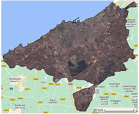
Casablanca is a vibrant city located in the western part of Morocco, situated on the Atlantic coast. Its geographical coordinates are approximately 33.5731° N latitude and 7.5898° W longitude. Figure 1 shows Casablanca area. As the largest city in Morocco and one of the major cities in North Africa, Casablanca serves as an essential economic, cultural, and industrial hub in the region.
The surrounding areas of Casablanca consist of suburbs, agricultural lands, and natural features, making it an ideal study area for assessing land cover dynamics and urban growth using satellite imagery.
Figure 1. Casablanca study area
3.2 Overview of Landsat 8 OLI satellite data used
The Landsat 8 OLI satellite data used in this study were acquired over multiple time periods, enabling temporal analysis to monitor changes in land cover over time. The spatial resolution of Landsat 8 OLI imagery ranges from 15 meters for the panchromatic band to 30 meters for the multispectral bands. Table 1 shows an overview of temporal and spatial resolution of Landsat 8.
Table 1. Spatial and temporal resolution of the Landsat 8 OLI imagery [24]
|
Name |
Spatial Resolution (Meters) |
Temporal Resolution |
|
B3 |
30 |
Landsat 8 orbits the Earth every 99 minutes, providing images with a high temporal frequency. |
|
B4 |
30 |
|
|
B5 |
30 |
|
|
B6 |
30 |
|
|
B7 |
30 |
Prior to analysis, the Landsat 8 OLI satellite data [24] underwent necessary preprocessing steps, such as atmospheric correction and radiometric calibration, to ensure data accuracy and reliability. These preprocessed images served as the foundational dataset for applying supervised algorithms [25] to classify land cover in the Casablanca region.
The Landsat 8 OLI satellite data, with its high-resolution and multispectral capabilities, provides a valuable resource for understanding land cover dynamics, urban expansion, and environmental changes in Casablanca, contributing to informed decision-making for sustainable development and resource management in the city.
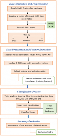
To achieve precise land cover classification in the designated study area, the methodology for using supervised algorithms in the classification satellite image within Google Earth Engine follows a systematic approach. By adhering to the process illustrated in Figure 2, researchers can effectively employ supervised machine learning algorithms, using Google Earth Engine, to classify Landsat satellite images. This facilitates the acquisition of valuable insights into land use dynamics, enabling informed decision-making in the realms of urban planning and environmental management. The procedural breakdown is as follows.
4.1 Data acquisition and preprocessing
The first step was to download Landsat 8 OLI satellite imagery [26] from the Google Earth Engine (GEE) [14] for the targeted region, Casablanca, Morocco. Subsequently, the imagery underwent preprocessing and filtering to rectify atmospheric distortions and ensure radiometric calibration, thereby guaranteeing data quality and consistency. The timeframe selected for analysis spanned from January 1, 2021, to December 31, 2021, capturing various land cover conditions and changes over the specified period.
Figure 2. Workflow of the methodology used
4.2 Data preparation and feature extraction
Following data acquisition, the process transitioned to data preparation and feature extraction. As shown in Table 2, five classes were defined based on study objectives and specific characteristics of the study area. Geometric points (features) were collected for each class from the composite image, and training data were generated by randomly partitioning this feature collection into 80% for training and 20% for validation.
4.3 Model training
At this stage, six supervised algorithms were chosen to undertake land cover classification, in correspondence with the six classes identified in the previous step (built-up, cultivated, forest, barren and aquatic areas). The algorithms, namely RF SVM [5], RF [6], GTB [7], DT [8], MD [9], and CART [8], were selected for implementation in the Google Earth Engine platform. The previously prepared data were used to train these algorithms, enabling them to learn to associate the extracted features with the corresponding land use classes. More specifically, the training data was divided into training and validation sets, in order to assess model performance during training and prevent over-fitting.
4.4 Model assessment
We measured the accuracy and generalization capabilities a model trained on the validation dataset. To assess the performance of each algorithm, evaluation measures such as accuracy and confusion matrices [27] were used. We followed a process to evaluate and calculate the accuracy of each classification method, i.e. the accuracy of a classified map. This process involves creating a set of random points from real terrain data sets, which we then compare to the classified data (classified map) using a confusion matrix. This matrix summarizes the prediction results for a specific classification problem, by comparing the actual data for a target variable with the model's predictions. Correct and incorrect predictions are identified and classified by class, enabling comparison with predefined values. The importance of this matrix lies in its ability to detect specific errors made by a prediction algorithm. Figure 3 shows an example of a confusion matrix, and Table 5 illustrates the kappa coefficient and overall accuracy for each classification.
Figure 3. Confusion matrix form [28]
4.5 Classification of land cover
The final phase of our study involved the creation of land-use maps and the visualization of results to assess model performance and identify classification errors and ambiguities. Based on the classification results, we generated detailed land use maps, assigning each pixel a specific land cover category. These maps provide an accurate visual representation of the spatial distribution of the different classes, facilitating an overall understanding of landscape dynamics in Casablanca.
The methodology used to classify Landsat satellite images in Casablanca using supervised algorithms via Google Earth Engine is systematic and structured. Data acquisition and preprocessing are involved in the process, in which Landsat 8 OLI imagery for Casablanca is obtained, preprocessed, and filtered to ensure data quality. The subsequent step includes data preparation and feature extraction, defining five land cover classes and creating training data for supervised algorithms such as Random Forest, CART, SVM, Decision Tree, MD, and GTB. Following the data preparation, the models are trained using the prepared training dataset, associating extracted features with corresponding land-use classes. Model evaluation is conducted using a validation dataset, employing accuracy and confusion matrices to assess the performance of each algorithm. This evaluation process is crucial in detecting specific errors made by the prediction algorithms. Finally, land cover classification is executed, resulting in the generation of land-use maps and visualization outputs for evaluating results and identifying any classification errors or ambiguities.
The outlined methodology provides a comprehensive framework for accurate land cover classification in the study area, facilitating valuable insights for urban planning and environmental management decisions.
Spectral indices, also known as spectral ratios, are mathematical formulas used in remote sensing and image analysis to extract specific information about the Earth's surface from satellite or aerial imagery [2]. These indices are designed to enhance certain features or characteristics that are not easily distinguishable in individual spectral bands [29].
They provide valuable insights for various applications, including agriculture, environmental monitoring, and urban planning. Table 1 shows the names of these bands and their spatial and temporal resolution.
·NIR: Near-Infrared band
·Red: Red band
·Green: Green band
·SWIR: Shortwave Infrared band.
Table 2. Equations of spectacles indices
|
Index Spectral |
Equation |
Description |
|
(NDVI) Normalized Difference Vegetation Index |
$\mathrm{NDVI}=\frac{\mathrm{NIR}-\mathrm{RED}}{\mathrm{NIR}+\mathrm{RED}}$ |
It is a widely used spectral index to assess vegetation health and density. It quantifies the abundance of healthy green vegetation by calculating the difference between near-infrared (NIR) and red spectral bands, divided by their sum. NDVI values range from -1 to +1, where positive values indicate healthy vegetation, zero represents non-vegetated surfaces like bare soil or water, and negative values indicate non-vegetated features like clouds or snow [30, 31]. |
|
(MNDWI) Modified Normalized Difference Water Index |
MNDWI$=\frac{\text { Green }- \text { SWIR1 }}{\text { Green }+ \text { SWIR1 }}$ |
It is used to identify and map water bodies and wet areas. It is an enhanced version of NDWI that uses the green and shortwave infrared (SWIR) bands. The formula involves calculating the difference between green and SWIR bands, divided by their sum. Higher MNDWI values suggest the presence of water, while lower values indicate land surfaces [32]. |
|
(BSI) Bare Soil Index |
$\mathrm{BSI}=\frac{\text { Green }+ \text { NIR }}{\text { Green }- \text { NIR }}$ |
It highlights areas with bare soil or unvegetated surfaces. It is calculated by using the SWIR and red bands to assess the presence of soil. The formula involves dividing the difference between SWIR and red bands by their sum, and then applying a quadratic function. Higher BSI values indicate bare soil or sparse vegetation, while lower values indicate dense vegetation [33]. |
|
(NDBI) Normalized Difference Built-up Index |
$\mathrm{NDBI}=\frac{\text { SWIR }- \text { NIR }}{\text { SWIR }+ \text { NIR }}$ |
It is used to detect and map built-up or urban areas. It compares the SWIR and NIR bands to identify built-up surfaces. The formula involves calculating the difference between SWIR and NIR bands, divided by their sum. Positive NDBI values suggest built-up areas, while negative values indicate non-built-up areas [34]. |
The experimental results highlight the varying performance of the different classification algorithms evaluated. Each of these algorithms presents strengths and weaknesses that merit in-depth analysis to guide the selection of the most appropriate model for specific applications. Figure 4 shows the overall accuracy (OA) of different methods.
Various metrics [35] have been used to assess the performance of each classification method [4], including overall accuracy, user accuracy for each class, manufacturer accuracy for each class and the Kappa coefficient obtained from the confusion matrix. The equations used to calculate these indicators are shown in Table 5. To assess the accuracy of classified land cover maps produced by supervised machine learning algorithms in GEE [11, 12].
We carried out an in-depth analysis of the confusion matrix for each method. The results are presented in Tables 3 and 4, which give a comprehensive overview of the accuracy assessment.
The confusion matrix is an essential tool for assessing the performance of a classification model [36], providing a detailed insight into how it classifies data according to its reality. It is generally square in shape, with the entries representing the different possible outcomes of a classification, as shown in Figure 3. In the case of a binary classification problem (with two classes), it is generally divided into four boxes [27]:
·True positives (VP): The model has correctly predicted that the element belongs to the positive class (actual and predicted values are both positive).
·True negatives (VN): The model has correctly predicted that the element does not belong to the positive class (actual and predicted values are both negative).
·False positives (FP): The model has incorrectly predicted that the element belongs to the positive class when it doesn't (actual value is negative and predicted is positive).
·False negatives (FN): The model has wrongly predicted that the element does not belong to the positive class, when in fact it does (actual value is positive and predicted is negative).
To improve the classification results, spectral indices such as NDVI [37], BSI, MNDWI and NDBI were incorporated. These indices were used during the feature extraction phase and included in the training data, helping to improve the classifier's performance. This approach enabled more accurate identification of land use categories.
Figure 4. Overall accuracy (OA) of different methods
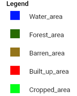
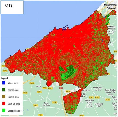
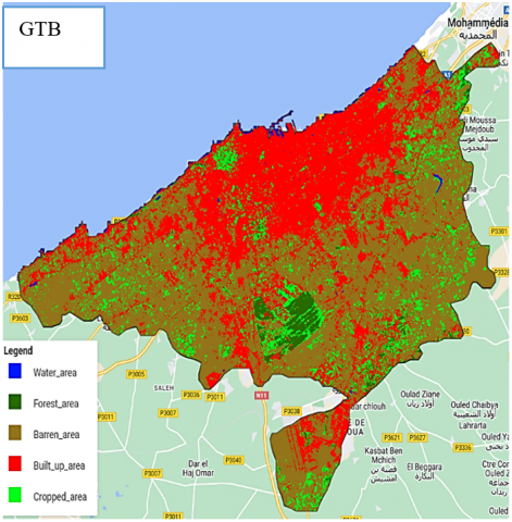
Figure 5. Legend of classification results
Random Forest clearly emerged as the leading algorithm, posting a remarkable overall accuracy of 95.42%. This high performance can be attributed to the ensemble nature of this model, which combines predictions from multiple decision trees to reduce over-fitting and improve generalization. This is particularly beneficial in complex contexts such as land cover classification. However, it is crucial to assess the model's sensitivity to variations in the training data, and to test its robustness in the face of different data sets. In addition, the impact of hyperparameters, such as the number of trees in the forest, should be examined to optimize model performance.
Minimum Distance also stands out, with an overall accuracy of 94.77%. Its strength lies in its conceptual simplicity and efficiency, particularly in class discrimination. However, the performance of this algorithm may be sensitive to the spatial distribution of the data and differences in class variability. Further analysis of the discriminating features identified by the MD could help to understand the underlying mechanisms of classification. It could also help identify scenarios where the simplicity of the MD approach might be preferable to more complex models.
Table 3. References data /classes
|
Classes |
Quantities of Geometric Points |
|
Water_area |
115 |
|
Barren_area |
150 |
|
Cropped_area |
119 |
|
Built-up_area |
130 |
|
Forest_area |
174 |
|
Total numbers |
688 |
Table 4. Land cover evaluation metrics of each method
|
Classification and Regression Trees (Cart) |
||||
|
|
Producer Accuracy |
User Accuracy |
Overall Accuracy |
Kappa coefficient |
|
Water_area |
100 |
100 |
91.50 |
0.89 |
|
Barren_area |
95.12 |
97.5 |
||
|
Forest_area |
89.65 |
81.25 |
||
|
Built-up_area |
76.92 |
83.33 |
||
|
Cropped_area |
92.30 |
92.30 |
||
|
Support Vector Machine (SVM) |
||||
|
|
Producer Accuracy |
User Accuracy |
Overall Accuracy |
Kappa coefficient |
|
Water_area |
100 |
100 |
83 |
0.78 |
|
Barren_area |
100 |
77.35 |
||
|
Forest_area |
82.75 |
75 |
||
|
Built-up_area |
69.23 |
81.81 |
||
|
Cropped_area |
50 |
86.66 |
||
|
Random Forest (RF) |
||||
|
|
Producer Accuracy |
User Accuracy |
Overall Accuracy |
Kappa coefficient |
|
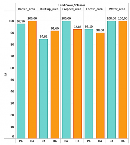
Water_area |
100 |
100 |
95.42 |
0.94 |
|
Barren_area |
97.56 |
100 |
||
|
Forest_area |
93.10 |
90 |
||
|
Built-up_area |
84.61 |
91.66 |
|
|
|
Cropped_area |
100 |
92.85 |
||
|
Gradient Tree Boost (GTB) |
||||
|
|
Producer Accuracy |
User Accuracy |
Overall Accuracy |
Kappa coefficient |
|
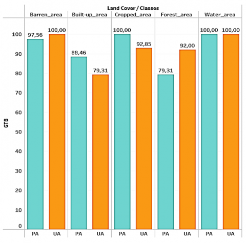
Water_area |
100 |
100 |
93.46 |
0.91 |
|
Barren_area |
97.56 |
100 |
||
|
Forest_area |
79.31 |
92 |
||
|
Built-up_area |
88.46 |
79.31 |
||
|
Cropped_area |
100 |
92.85 |
||
|
Decision Trees (DT) |
||||
|
|
Producer Accuracy |
User Accuracy |
Overall Accuracy |
Kappa coefficient |
|
Water_area |
100 |
100 |
91.50 |
0.89 |
|
Barren_area |
95.12 |
97.5 |
||
|
Forest_area |
89.65 |
81.25 |
||
|
Built-up_area |
76.92 |
83.33 |
||
|
Cropped_area |
92.30 |
92.30 |
||
|
Minimum Distance (MD) |
||||
|
|
Producer Accuracy |
User Accuracy |
Overall Accuracy |
Kappa coefficient |
|
Water_area |
100 |
100 |
94.77 |
0.93 |
|
Barren_area |
95.12 |
100 |
||
|
Forest_area |
86.20 |
92.59 |
||
|
Built-up_area |
92.30 |
88.88 |
||
|
Cropped_area |
100 |
89.65 |
||
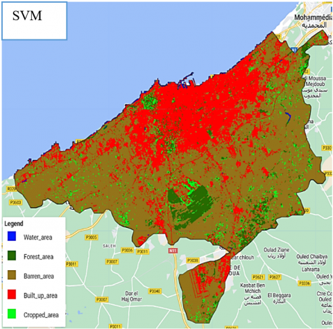
Figure 6. Land cover classification map for Casablanca
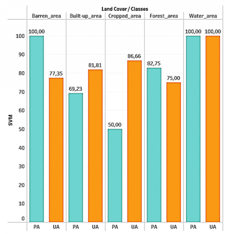
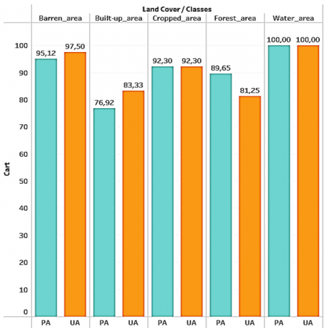
Figure 7. The producer’s accuracy (PA), and the user’s accuracy (UA) values of each classifier
Table 5. Kappa coefficient and overall accuracy for land use classification of each classifier used
|
Classifier |
Overall Accuracy % |
Kappa Coefficient |
|
SVM |
83 |
0.78 |
|
Cart |
91.50 |
0.89 |
|
RF |
95.42 |
0.94 |
|
GTB |
93.46 |
0.91 |
|
DT |
91.50 |
0.89 |
|
MD |
94.77 |
0.93 |
Table 6. Equations of evaluation metric
|
Metrics |
Equation |
|
(PA) Producer Accuracy |
PA $=\frac{\text { Correct imprevious surface pixel }}{\text { Total imprevious pixels }}$ |
|
Kappa Coefficient |
$K=\frac{\mathrm{p}_{\text {accord }}-\mathrm{P}_{\text {Hasard }}}{1-\mathrm{P}_{\text {Hasard }}}$ |
|
(OA) Overall Accuracy |
$\mathrm{OA}=\frac{\text { Number of correctly classified samples }}{\text { Number of samples }}$ |
|
(UA) User Accuracy |
$\mathrm{UA}=\frac{\text { Correct imprevious surface pixel }}{\text { Correct }+ \text { Misclassified pixel }}$ |
Although the SVM achieved 100% accuracy for the "Water" class, its overall accuracy of 83% raises questions about its ability to handle variability in other classes. SVM is renowned for its ability to handle high-dimensional data, but its success often depends on the judicious choice of kernels and parameters. A thorough analysis of support vectors and separation margin could reveal information about the relative difficulty of classification for different classes. Optimization of SVM parameters could also be explored to improve its performance.
Gradient Tree Boost presents an interesting balance between producer and user accuracy, with an overall accuracy of 93.46%. This algorithm can adjust its predictions based on previous errors, which can be advantageous in scenarios where classes are unbalanced. However, GTB's interpretability may be less than that of other, simpler algorithms, raising questions about the model's transparency. For applications where model explicability is crucial, GTB-specific interpretation techniques could be explored [7].
Decision trees (CART and DT) have shown solid performance, albeit inferior to that of RF. Their simplicity and interpretability make them attractive candidates in contexts where understanding the decision process is crucial. However, the propensity of decision trees to overfitting can be a challenge, and regularization techniques may be needed to improve their generalizability. The use of cross-validation and other model validation strategies could help alleviate this problem. Table 3 and 4 illustrate the Kappa coefficient and Overall accuracy for land use classification of each classifier used.
Integrating the results of previous studies [3, 19, 22, 26, 37-42] and our own research, the main achievement of this study lies in the successful adaptation of the methodology to land use mapping and evaluation in different geographical contexts.
The results underline the superiority of the Random Forest classifier over other classifiers, with an impressive accuracy of 95.42% and a Kappa coefficient of 0.94, underscoring its substantial superiority over random classification. Figure 5 shows the legend of classification results and Figure 6 gives a visual presentation of the classified cards.
In summary, this research has contributed significantly by successfully adapting the methodology for mapping and assessing land use in diverse regions or countries. The results underlined the importance of spectral indices in improving classification accuracy and highlighted the need to consider the inherent complexity of land cover classification in diverse contexts. Figure 7 shows the producer’s accuracy (PA), and the user’s accuracy (UA) values of each classifier.
In conclusion, this paper has embarked on a comprehensive exploration of the effectiveness of six supervised algorithms in the classification satellite images, specifically within the dynamic urban landscape of Casablanca, Morocco. The selected algorithms, including Random Forest, Classification and Regression Trees, Support Vector Machine, Decision Trees, Minimum Distance, and Gradient Tree Boost, were implemented on the Google Earth Engine platform, leveraging its computational capabilities. This study produced significant results, highlighting the superiority of the Random Forest classifier in land use mapping in Casablanca, with an accuracy of 95.42% and a Kappa coefficient of 0.94. The integration of spectral indices, such as NDVI and BSI, considerably improved classification accuracy, demonstrating the relevance of this approach in a variety of contexts. These results are of crucial importance for the accurate mapping of urban areas, with practical implications for resource management and urban planning. The real-world applications of this research can be seen in the increased ability to understand and monitor changes in land use, particularly in areas such as natural resource management, disaster prevention and urban planning decision-making. The spectral indices used in this study offer a promising approach to discriminating different land cover characteristics, paving the way for more specific applications such as early detection of changes in forest areas or monitoring of expanding urban areas.
For future work, it is recommended to further explore the use of new data sources, including higher resolution satellite images, as well as emerging techniques such as deep learning. The exploration of hybrid methods, combining supervised and unsupervised approaches, could also help improve the robustness of classification models. In addition, the integration of temporal data could provide a deeper understanding of seasonal and long-term changes in land cover. These recommendations are aimed at further optimizing the accuracy of classifications and extending the scope of applications in fields such as environmental management and urban change monitoring.
[1] Ouchra, H., Belangour, A., Erraissi, A. (2022). Satellite data analysis and geographic information system for urban planning: A systematic review. In 2022 International Conference on Data Analytics for Business and Industry (ICDABI), Sakhir, Bahrain, pp. 558-564. https://doi.org/10.1109/ICDABI56818.2022.10041487
[2] Ouchra, H., Belangour, A. (2021). Satellite image classification methods and techniques: A survey. In 2021 IEEE International Conference on Imaging Systems and Techniques (IST), Kaohsiung, Taiwan, pp. 1-6. https://doi.org/10.1109/IST50367.2021.9651454
[3] Ouchra, H., Belangour, A., Erraissi, A. (2023). Machine learning algorithms for satellite image classification using Google Earth Engine and Landsat satellite data: Morocco case study. IEEE Access, 11: 71127-71142. https://doi.org/10.1109/ACCESS.2023.3293828
[4] Ouchra, H., Belangour, A., Erraissi, A. (2022). Machine learning for satellite image classification: A comprehensive review. In 2022 International Conference on Data Analytics for Business and Industry (ICDABI), Sakhir, Bahrain, pp. 1-5. https://doi.org/10.1109/ICDABI56818.2022.10041606
[5] Awad, M. (2021). Google earth engine (GEE) cloud computing based crop classification using radar, optical images and Support Vector Machine Algorithm (SVM). In 2021 IEEE 3rd International Multidisciplinary Conference on Engineering Technology (IMCET), Beirut, Lebanon, pp. 71-76. https://doi.org/10.1109/IMCET53404.2021.9665519
[6] Magidi, J., Nhamo, L., Mpandeli, S., Mabhaudhi, T. (2021). Application of the random forest classifier to map irrigated areas using google earth engine. Remote Sensing, 13(5): 876. https://doi.org/10.3390/RS13050876
[7] Natekin, A., Knoll, A. (2013). Gradient boosting machines, a tutorial. Frontiers in Neurorobotics, 7: 21. https://doi.org/10.3389/fnbot.2013.00021
[8] Hu, Y., Dong, Y. (2018). An automatic approach for land-change detection and land updates based on integrated NDVI timing analysis and the CVAPS method with GEE support. ISPRS Journal of Photogrammetry and Remote Sensing, 146: 347-359. https://doi.org/10.1016/J.ISPRSJPRS.2018.10.008
[9] Borra, S., Thanki, R., Dey, N. (2019). Satellite Image Analysis: Clustering and Classification. Singapore: Springer. https://doi.org/10.1007/978-981-13-6424-2
[10] Ouchra, H., Belangour, A., Erraissi, A. (2022). Spatial data mining technology for GIS: A review. In 2022 International Conference on Data Analytics for Business and Industry (ICDABI), Sakhir, Bahrain, pp. 655-659. https://doi.org/10.1109/ICDABI56818.2022.10041574
[11] Ouchra, H., Belangour, A., Erraissi, A. (2022). A comprehensive study of using remote sensing and geographical information systems for urban planning. Internetworking Indonesia Journal, 14(1): 15–20.
[12] Ouchra, H., Belangour, A., Erraissi, A. (2023). An overview of GeoSpatial Artificial Intelligence technologies for city planning and development. 2023 Fifth International Conference on Electrical, Computer and Communication Technologies (ICECCT), Erode, India, pp. 1-7. https://doi.org/10.1109/ICECCT56650.2023.10179796.
[13] Yang, L., Driscol, J., Sarigai, S., Wu, Q., Chen, H., Lippitt, C.D. (2022). Google Earth Engine and artificial intelligence (AI): A comprehensive review. Remote Sensing, 14(14): 3253. https://doi.org/10.3390/RS14143253
[14] Gorelick, N., Hancher, M., Dixon, M., Ilyushchenko, S., Thau, D., Moore, R. (2017). Google Earth Engine: Planetary-scale geospatial analysis for everyone. Remote Sensing of Environment, 202: 18-27. https://doi.org/10.1016/J.RSE.2017.06.031
[15] Ma, L., Li, M.C., Ma, X.X., Cheng, L., Du, P.J., Liu, Y.X. (2017). A review of supervised object-based land-cover image classification. ISPRS Journal of Photogrammetry and Remote Sensing, 130: 277–293. https://doi.org/10.1016/j.isprsjprs.2017.06.001.
[16] Shafaey, M.A., Salem, M.A.M., Ebied, H.M., Al-Berry, M.N., Tolba, M.F. (2018). Deep learning for satellite image classification. In International Conference on Advanced Intelligent Systems and Informatics, Springer, Cham, pp. 383-391. https://doi.org/10.1007/978-3-319-99010-1_35
[17] Ouchra, H., Belangour, A. (2021). Object detection approaches in images: A weighted scoring model based comparative study. International Journal of Advanced Computer Science and Applications, 12(8): 268-275.
[18] Ouchra, H., Belangour, A., Erraissi, A. (2022). A comparative study on pixel-based classification and object-oriented classification of satellite image. International Journal of Engineering Trends and Technology, 70(8): 206-215. https://doi.org/10.14445/22315381/IJETT-V70I8P221
[19] Niknejad, M., Zadeh, V.M., Heydari, M. (2014). Comparing different classifications of satellite imagery in forest mapping (Case study: Zagros forests in Iran). International Research Journal of Applied and Basic Sciences, 8(9): 1407-1415.
[20] Firozjaei, M. K., Daryaei, I., Sedighi, A., Weng, Q.H., Panah, S.K. (2019). Homogeneity Distance Classification Algorithm (HDCA): A novel algorithm for satellite image classification. Remote Sens (Basel), 11(5): 546. https://doi.org/10.3390/rs11050546.
[21] Mahyoub, S., Rhinane, H., Fadil, A., Mansour, M., Saleh, M., Al-Nahmi, F. (2020). Using of open access remote sensing data in google earth engine platform for mapping built-up area in Marrakech City, Morocco. In 2020 IEEE International conference of Moroccan Geomatics (Morgeo), Casablanca, Morocco, pp. 1-5. https://doi.org/10.1109/MORGEO49228.2020.9121912
[22] Sellami, E.M., Rhinane, H. (2023). A new approach for mapping land use/land cover using google earth engine: A comparison of composition images. The International Archives of the Photogrammetry, Remote Sensing and Spatial Information Sciences, 48: 343-349. https://doi.org/10.5194/isprs-archives-XLVIII-4-W6-2022-343-2023.
[23] Chemchaoui, A., Brhadda, N., Alaoui, H.I., Rabea, Z. (2023). Accuracy assessment and uncertainty of the 2020 10-meter resolution land use land cover maps at local scale. Case: Talassemtane National Park, Morocco. https://doi.org/10.21203/rs.3.rs-2953599/v2
[24] Loyd, C. (2013). Landsat 8 Bands | Landsat Science (no date a). Available at: https://landsat.gsfc.nasa.gov/satellites/landsat-8/landsat-8-bands/#, accessed on 26 October 2023.
[25] Ouchra, H., Belangour, A. (2021). Object detection approaches in images: A survey. In Thirteenth International Conference on Digital Image Processing (ICDIP 2021), 11878: 132-141. https://doi.org/10.1117/12.2601452
[26] Jamali, A. (2019). Evaluation and comparison of eight machine learning models in land use/land cover mapping using Landsat 8 OLI: A case study of the northern region of Iran. Machine Learning, 1(11): 1448. https://doi.org/10.1007/s42452-019-1527-8
[27] Heydarian, M., Doyle, T.E., Samavi, R. (2022). MLCM: Multi-label confusion matrix. IEEE Access, 10: 19083-19095. https://doi.org/10.1109/ACCESS.2022.3151048
[28] Emilion, P.M. (2023). Matrice de confusion: Comment la lire et l’interpréter? https://www.jedha.co/formation-ia/matrice-confusion, accessed on 13 December 2022.
[29] Bouzekri, S., Lasbet, A.A., Lachehab, A. (2015). A new spectral index for extraction of built-up area using Landsat-8 data. Journal of the Indian Society of Remote Sensing, 43: 867-873. https://doi.org/10.1007/S12524-015-0460-6
[30] Yengoh, G.T., Dent, D., Olsson, L., Tengberg, A.E., Tucker III, C.J. (2015). Use of the normalized difference vegetation index (NDVI) to assess land degradation at multiple scales: Current status, future trends, and practical considerations. Springer. https://doi.org/10.1007/978-3-319-24112-8
[31] Gascon, M., Cirach, M., Martínez, D., Dadvand, P., Valentín, A., Plasència, A., Nieuwenhuijsen, M.J. (2016). Normalized difference vegetation index (NDVI) as a marker of surrounding greenness in epidemiological studies: The case of Barcelona city. Urban Forestry & Urban Greening, 19: 88-94. https://doi.org/10.1016/J.UFUG.2016.07.001
[32] Mfondoum, A.H.N., Etouna, J., Nongsi, B.K., Moto, F.A.M., Deussieu, F.N. (2016). Assessment of land degradation status and its impact in arid and semi-arid areas by correlating spectral and principal component analysis neo-bands. International Journal of Advanced Remote Sensing and GIS, 5(2): 1539-1560. https://doi.org/10.23953/CLOUD.IJARSG.77
[33] Abutaleb, K., Ngie, A., Darwish, A., Ahmed, M., Arafat, S., Ahmed, F. (2015). Assessment of urban heat island using remotely sensed imagery over Greater Cairo, Egypt. Advances in Remote Sensing, 4(1): 35-47. https://doi.org/10.4236/ARS.2015.41004
[34] NDBI (2023). An overview of the Spatial Analyst functions. at: https://pro.arcgis.com/en/pro-app/latest/arcpy/spatial-analyst/ndbi.htm, accessed on 19 May 2023.
[35] Ghaderizadeh, S., Abbasi-Moghadam, D., Sharifi, A., Tariq, A., Qin, S. (2022). Multiscale dual-branch residual spectral–spatial network with attention for hyperspectral image classification. IEEE Journal of Selected Topics in Applied Earth Observations and Remote Sensing, 15: 5455-5467. https://doi.org/10.1109/JSTARS.2022.3188732
[36] Nehzak, H. K., Aghaei, M., Mostafazadeh, R., Rabiei-Dastjerdi, H. (2022). Assessment of machine learning algorithms in land use classification. In Computers in Earth and Environmental Sciences, Elsevier. pp. 97–104. https://doi.org/10.1016/B978-0-323-89861-4.00022-1
[37] Bellón B, Bégué A, Lo Seen D, De Almeida CA, Simões M. (2017). A remote sensing approach for regional-scale mapping of agricultural land-use systems based on NDVI time series. Remote Sensing, 9(6): 600. https://doi.org/10.3390/RS9060600
[38] Zurqani, H.A., Post, C.J., Mikhailova, E.A., Allen, J.S. (2019). Mapping urbanization trends in a forested landscape using Google Earth Engine. Remote Sensing in Earth Systems Sciences, 2: 173-182. https://doi.org/10.1007/s41976-019-00020-y
[39] Sharifi, A. (2020). Flood mapping using relevance vector machine and SAR Data: A case study from Aqqala, Iran. Journal of the Indian Society of Remote Sensing, 48(9): 1289–1296. https://doi.org/10.1007/S12524-020-01155-Y
[40] Masoumi, F., Eslamkish, T., Honarmand, M., Abkar, A. A. (2017). A comparative study of landsat‐7 and landsat‐8 data using image processing methods for hydrothermal alteration mapping. Resource Geology, 67(1): 72-88. https://doi.org/10.1111/rge.12117
[41] Bachri, I., Hakdaoui, M., Raji, M., Teodoro, A.C., and Benbouziane, A. (2019). Machine learning algorithms for automatic lithological mapping using remote sensing data: A case study from Souk Arbaa Sahel, Sidi Ifni Inlier, Western Anti-Atlas, Morocco. ISPRS Int J Geoinf, 8(6): 248. https://doi.org/10.3390/ijgi8060248
[42] Idoumskine, I., Aydda, A., Ezaidi, A., Althuwaynee, O. F. (2022). Assessing land use/land cover change using multitemporal landsat data in Agadir City (Morocco). In Distributed Sensing and Intelligent Systems: Proceedings of ICDSIS 2020, Springer, Cham, 337-350. https://doi.org/10.1007/978-3-030-64258-7_30