Application of the ITS-UCD Model for the Assessment of CO2 Compression and Transport Costs for the Simeri Crichi - Botricello1 Route in a Theoretical CCS Retrofit Project of the Simeri Crichi Thermal Power Plant

Luca Rosati* | Angelo Spena | Fedora Quattrocchi
OPEN ACCESS
The power plant of Simeri Crichi (Calabria Region, Italy) under study was already managed by Edison S.p.A. and it is fueled by natural gas. This study is dealing with the hypothesis to perform a retrofit device of the plant, with the addition of a standard “CO2 Capture”, able to perform a capture rate up to 90%; it has been proposed here the sizing of the compression station and the pipeline which connects the plant to the injection site Botricello 1, studied in the frame of a gross screening of the storage sites in the Calabria Region in Italy.
This study took into account the costs of construction, operation and maintenance (O&M) of both the compression plant and the sound pipeline.
Eventually, an estimation of the gross static storage capacity of the Botricello1 reservoir is provided.
carbon capture and storage, power plants, greenhouse gasses, cost assessment
In December 2015, at COP 21 in Paris, 195 Countries signed the Paris Climate Agreement [1]. The long-term climate goals of the agreement were defined as:
So far, global climate models have not been able to achieve really useful results for the reduction of greenhouse gases from the atmosphere and/or economically advantageous/sustainable while remaining consistent with the objectives of the 2015 Paris Agreement, without taking into account critical technologies such as CCS (Carbon Capture & Storage), bioenergy and their combination (BECCS) [2].
The gap between the global efforts currently underway and the emissions reductions needed to reach the 2℃ target agreed in Paris is immense. It requires approximately 760 gigatonnes (Gt) of CO2 emissions reduction across the energy sector between now and 2060 [2].
Although the transition from fossil fuels to renewable sources is concrete and indisputable, the statistics and projections propose scenarios still characterized by an important presence of natural gas and coal in the field of electricity generation, from now to the next 20 years.
The IEA estimates a flat trend in global coal demand; this in an expanding energy system means a very modest decline in the demand for coal which will rise from the current 27% to 21% in 2040 considering the current energy policies implemented by the various countries.
Even considering the Sustainable Development Scenario as far as the reduction is estimated to be 60% lower than that relating to current policies, the IEA estimates a coal demand of still around 1771 Mtce (metric tonnes carbon equivalent) in 2040.
Although coal demand has fallen in China - by far the world's largest coal consumer - due in large part to a strong political push to improve air quality, by other Asian developing countries the use of coal shows no sign of diminishing. This is because of the need for these countries to increase their use of coal to meet the rapidly growing demand for electricity and industrial development [3].
As for natural gas, there has been a "gas rush" in many countries in recent years and natural gas now accounts for over 20% of global electricity production, with more power plants planned for construction (despite the natural gas “peak” is foreseen to be in few decades). The main reason is linked to the characteristic of natural gas to be the cleanest fossil fuel: the CO2 (per unit of energy produced) released into the atmosphere is in fact 40% lower than coal and 20% lower than oil.
Suffice it to say that China has almost increased the consumption of natural gas in the last 20 years from 28 bcm (billion cubic meters) in the early 2000s to 268 bcm in 2018 with a growth trend that estimates gas consumption in 2030 at 553 bcm [4].
However, it must be considered that although a gas-fired powerplant is considered "cleaner" than a coal-fired one, it is far from low carbon: a combined cycle plant has an emission profile of approximately 370 grams of CO2 per kilowatt hour (g CO2 / KWh) compared to about 700 g CO2 / KWh for an ultra-supercritical coal-fueled powerplant) [5].
Considering the SDS scenario (Suistainable Development Scenario), it is estimated an important production of electric energy by gas-fired powerplants retrofitted with CCS. It is estimated a potential of more than 2 Gt of CO2 captured cumulatively by 2040; this means 160 GW of gas-fired power plants equipped with CCS that will supply around 900 TWh of global energy generation equivalent to one-sixth of the total production of energy from gas.The present study carried out with the aim of proposing a possible solution for the conversion to CCS of Italian gas-fired power stations, now without this technology, fits into this context, from the moment in which following the tightening of CO2 emissions regulations, also this type of power plant will have to be converted mandatorily with CCS [2].
The Edison plant of Simeri Crichi is located South-East of the municipality of Catanzaro at an approximate distance of 7 km, and about 4 km from the Ionian coast. Located at an altitude of approximately 36 m a.s.l., it is located in a valley, between the hydrographic left of the Alli river and the Provincial Road 16 (SP) of Bonifica Alli - Punta della Castella.
The power plant fueled exclusively by natural gas, is of the combined cycle type with gross nominal electric power, in pure condensation structure, equal to approximately 857.4 MWe at the reference conditions for the site in question (15℃, 1009 mbar, 60% relative humidity). The plant essentially consists of two heavy duty gas turbines (TG1 and TG2) with a nominal electric power of approximately 277.4 MW.
Both groups feed a steam turbine (302.53 MWe) connected to an alternator and further thermal users. The electricity produced net of self-consumption is completely fed into the grid managed by Terna. Lastly, the plant is designed for the supply of thermal energy in the form of steam to any future external users (for a power supplied equal to 60 MW), in accordance with what is specified in the authorization for the construction and operation of the power plant issued by the Municipality of Simeri Crichi on March 8, 2004 [6].
The data of interest are shown in Table 1.
Table 1. Characteristics of the Simeri Crichi power plant
|
Power plant capacity |
857 MW |
|
CO2 emissions p.c. |
3,884 t/d |
|
CO2 emissions p.c. |
1,417,549 t/y |
2.1 Compression power calculation
After its separation from the flue gases emitted from a power plant or an energy complex, the CO2 must be compressed starting from atmospheric pressure (Pin = 0.1 MPa), the pressure at which it exists as a gas, up to a pressure suitable for the transport on pipeline (generally Pfi = 10-15 MPa), pressure at which CO2 is liquid or in the "dense phase" region, depending on its temperature. Depending on the phase of the CO2, a compressor is used when it is in the gas phase, while when it is in the liquid / dense phase, a pump must be used. It can be assumed that the cut-off pressure (Pcut-off) at which we have the switch from the compressor to the pump is the critical CO2 pressure: 7.38 MPa [7].
Table 2. Pressure values considered for the compression plant project
|
Pin |
0.1 MPa |
|
Pcut-off |
7.38 MPa |
|
Pfi |
10-15 MPa |
$C R=\left(\frac{P_{\text {cut-off }}}{P_{\text {in }}}\right)^{\frac{1}{N_{\text {stage }}}}$ (1)
The next step is the calculation of the power required for compression in each stage (Ws, i) through the Eq. (2):
$W_{s, i}=\frac{1000}{24 * 3600} * \frac{m Z_{s} R T_{i n}}{M \eta_{i s}} * \frac{K_{s}}{K_{s}-1}+\left(C R^{\frac{K_{s}-1}{K_{s}}}-1\right)$ (2)
where:
-R = 8,314 [kJ/(kmol*K)];
-M = 44,01 [kg/kmol];
-Tin = 313,15 [K];
-ηis = 0.8;
-1000 indicates the kg in one ton;
-24 indicated the hours in one day;
-3600 indicates the seconds in one hour;
-m indicates the CO2 mass flow rate in [tons/day].
Table 3. Pressure, Zs, Ks values for each stage of the compression plant
|
Stage |
Pressure step |
Zs |
Ks |
|
1 |
0.1 – 0.24 MPa |
0.995 |
1.277 |
|
2 |
0.24 – 0.56 MPa |
0.985 |
1.286 |
|
3 |
0.56 – 1.32 MPa |
0.970 |
1.309 |
|
4 |
1.32 – 3.12 MPa |
0.935 |
1.379 |
|
5 |
3.12 – 7.38 MPa |
0.845 |
1.704 |
The required powers, calculated for each stage, must then be added together to obtain the total power required by the compressor (Ws-total). According to the IEA GHG PH4 / 6 report, the maximum size of a series of compressors built according to modern technologies is 40000 kW, which is why if the total power required by the compressor is greater than this threshold, the CO2 flow rate and the power request must be distributed in a "train" of compressors in series arranged in parallel. The number of compressor series must obviously be an integer and is calculated through the Eq. (3):
$N_{\text {train }}=R O U N D_{U P} *\left(\frac{W_{s-\text { total }}}{40,000}\right)$ (3)
The power required for pumping is obtained through the Eq. (4):
$W_{p}=\frac{1000 * 10}{24 * 36} * \frac{m *\left(P_{f i}-P_{\text {cut-off }}\right)}{\rho * \eta_{p}}$ (4)
where:
-m = CO2 mass flow rate in [tons/day];
-ρ = CO2 density, 630 kg/m3;
-ηp = 0.75;
-1000 = kg in one ton;
-24 = hours in one day;
-10 = pressure in bar corresponding one MPa;
-36 = (m3 * bar)/(hr * kW).
Once the power required by the pump has also been calculated, we can calculate the total power required for CO2 compression.
The dependence of the power required for the flow rate compression is linear, both in the case of the compressor and in the case of the pump; however, the power required for pumping is lower than that required for compression, due to the fact that the compressor increases the CO2 pressure from 0.1 to 7.38 MPa (with a compression ratio equal to 73.8), while the pump increases the pressure from 7.38 to 10 MPa (with a compression ratio of only 2). Following the model proposed by McCollum, a 5-stage system was hypothesized, each interspersed with water-cooled inter-cooling. The presence of intercooling is of fundamental importance also because in this way, at each stage, it is possible to separate the condensate (to minimize the presence of water in the CO2 flow, which could be the cause, together with carbon dioxide, of corrosive processes).
The compression is then performed from atmospheric pressure (exiting from the capture system) up to the critical pressure (about 73 bar) through the use of a five-stage compressor.
The CO2 is subsequently sent to an intermediate tank (which acts as a separator) from which, eventually, it will be sent to the pump used for compression up to the pressure chosen for entry into the pipeline. Considering a daily mass flow rate of 3,495.3 tons/day equal to 40.45 kg/s, a summary scheme of the system simulation is given where, as can be seen from the values, the overall power used by the compression is equal to 14.6 MW while the power used by the pump to arrive from critical conditions to those optimized for entry into the pipeline (10 Mpa) is much less (about 224 KW).
Table 4. Results of the sizing of the compression plant
|
N° compression stages |
5 |
|
Mass flow rate (m) |
3,495.33 t/d |
|
Pinitial |
0.1 Mpa |
|
Pcut-off |
7.38 Mpa |
|
Pfinal |
10 Mpa |
|
Compressor Ratio (CR) |
2.36 |
|
Wstage,1 |
3,002.85 KW |
|
Wstage,2 |
2,979.91 KW |
|
Wstage,3 |
2,952.39 KW |
|
Wstage,4 |
2,895.50 KW |
|
Wstage,5 |
2,785.34 KW |
|
Wcompressor-total |
14,615.98 KW |
|
his |
0.80 |
|
hp |
0.75 |
|
Wpump |
224.32 KW |
2.2 Investment costs, operation and maintenance costs, levelized costs
The investment (capital), operating and maintenance (O&M) costs and the normalized costs per ton of compressed carbon dioxide were calculated starting from the power required for compression.
Compression capital costs, obtained from McCollum & Odgen, are expressed by the Eq. (5):
$\mathrm{C}_{\text {comp }}=\mathrm{m}_{\text {train }} \mathrm{N}_{\text {train* }}\left[\left(0.13 * 10^{6}\right) *\left(\mathrm{~m}_{\text {train }}\right)^{-0.71}++\left(1.40 * 10^{6}\right) *\left(\mathrm{~m}_{\text {train }}\right)^{-0.60} * \ln \left(\frac{\mathrm{P}_{\text {cut-off }}}{\mathrm{P}_{\text {Pinitial }}}\right)\right]$ (5)
The capital cost relative to the pumping can then be calculated through Eq. (6):
$\mathrm{C}_{\text {pump }}=\left\{\left(1.11 * 10^{6}\right) *(W p / 1000)\right\}+0.07 * 10^{6}$ (6)
Once the two cost items were added together, in order to calculate the annual costs, the CRF factor was introduced. Annual costs are expressed by the Eq. (7):
$C_{\text {annual }}=C_{\text {total }} * C F R$ (7)
where, CRF is the Capital Recovery Factor, a sort of annual amortization rate that takes into account the useful life of the project and which is taken on average equal to 0.15 (McCollum & Odgen). In order to calculate the real mass flow rate of compressed CO2, the daily flow rate was multiplied for 365 days, taking into account a "Capacity Factor" equal to 0.85, considering the plant active for 85% of the time. Regarding the levelized costs, the annual compression and pumping cost was simply divided by the annual amount of CO2 compressed (tons).
Table 5. Compression costs
|
Capital cost (compression) |
33,481,877.38 € |
|
Capital cost (pumping) |
398,016.24 € |
|
Total capital cost |
33,879,893.62 € |
|
Annualized capital cost |
5,081,984.04 € |
|
CO2 mass flow rate |
1,084,424.89 tons/year |
|
Levelized capital cost |
4.69 €/tonne |
Annual O&M costs were considered by McCollum & Odgen to be equal to 4% of the capital cost.
Table 6. O&M costs
|
O&M factor |
0.04 € |
|
O&M annual cost |
1,355,195.74 € |
|
O&M levelized cost |
1.25 €/tonne |
$E_{\text {annual }}=E_{\text {comp }}+E_{\text {pump }}=p e *\left(W_{s-\text { total }}+W_{p}\right) *$
$(C F * 24 * 365)$ (8)
Table 7. Electricity costs
|
Electricity price |
0.07 € |
|
O&m annual cost |
7,956,063.49 € |
|
O&M levelized cost |
7.34 €/tonne |
Summarizing the total costs as a sum of the three components, as shown in the Eq. (9), we obtain the values shown in Table 8:
Ctot = Ccapital + CO&M + Celectricity (9)
Table 8. Total costs of compression
|
Total annual cost |
14,393,243.28 € |
|
Total levelized cost |
13.27 €/ton |
All costs have been discounted to 2020.
3.1 Pipeline design
During the pipeline design phase, we tried to minimize the overall cost of the work considering the cost of the pipeline and the compression plant as a reference (both in terms of investment cost and operating cost during the entire estimated lifetime for the project, since the first costs are fundamental in the pipeline while the second are predominant in the compression plant).
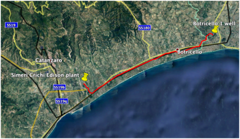
Regarding the route that connects the plant to the Botricello 1 injection well, we tried to identify the shortest way, avoiding infrastructure and residential areas as much as possible and possibly skirting a viable road for means of transport to limit the costs for moving of all the materials necessary for the realization and for future ordinary or extraordinary maintenance.
We also tried to avoid going from a lower to a higher elevation in order not to have to resort to a recompression plant, which entails a considerable increase in costs.
Regarding the choice of materials, for reasons of compatibility with the components of the gas that flows through the pipeline,
CO2 pipelines are usually built using carbon steel, for the use of which it is however necessary to comply with certain specifications and operating conditions. This material was also chosen because of its characteristic of being able to withstand up to -80℃, the temperature reached in the event of depressurization.
Since the CO2 before entering the pipeline undergoes a drying process, it can be considered non-corrosive. Under these conditions it is therefore not necessary to protect the pipeline internally from corrosion.
Externally, however, due to the atmospheric agents and the composition of the soil where the pipeline is buried, it must be protected with a coating that ensures its protection from corrosion as an alternative to the more complicated cathodic protection and made of HDPE (High Polyethylene Density).
As mentioned, the design of the pipeline was based on a technical and economic evaluation with the aim of minimizing investment and operating costs.
In this regard, the evaluation of the diameter of the pipeline is fundamental as it is a function of the pressure loss along the pipeline itself which in turn influences the choice of the compression system.
The pipeline pressure drop can be calculated using the Eq. (10) [7]:
$\Delta \mathrm{P}=\lambda *(L / D) *(1 / 2) * \rho * \mathrm{v}^{2}$ (10)
where:
In the above flow equation, the velocity term, v, is a function of the mass flow rate and the cross-sectional area (i.e., diameter) of the pipeline.
Figure 1. The chosen route, taken from the Google Earth Pro software
Thus, the Eq. (10) can be rearranged to form the Eq. (11):
$D^{5}=\left(8 * \lambda * m^{2}\right) /\left(\pi^{2} * \rho * \Delta \mathrm{P} /_{L}\right)$ (11)
where:
m = CO2 mass flow rate.
Key data used for the calculation are:
Based on the previous analyzes and considerations, the evaluation carried out has led to the results illustrated in the following graphs, where to each diameter considered for the analysis is associated the corresponding pressure drop between inlet and outlet, as a function of the density variation (in turn linked to the variation in temperature) and the length of the section.
According to this value, it is therefore possible to go back, since the minimum outlet pressure of the pipeline had previously been set, to the required inlet pressure for the pipeline (and therefore of fundamental importance for the compression plant).
Figure 2. Pressure drop as a function of the pipeline’s diameter
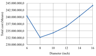
As previously anticipated, the final choice of the diameter of the two sections under consideration was made according to a technical-economic optimization.
With the choice of diameter, we tried to minimize the overall costs of the compression-transport section of the present project.
It must be considered, in fact, that as the diameter increases, there is a decrease in pressure losses and therefore consequently a decrease in pressure drop along the pipeline as well as of the cost of the compression plant, but at the same time the cost of construction of the pipeline increases.
Based on these assessments, and using a series of economic models (which will be shown in the following paragraph) to evaluate the aforementioned costs, the value of the diameter that optimizes this analysis has been reached.
Figure 3. Total investment cost as a function of pipeline’s diameter
The analysis of the graphs presented shows that the diameter that optimizes the analysis conducted is that of 10 inches (10 Mpa).
3.2 Investment costs, operation and maintenance costs, levelized costs [7]
The capital costs have been calculated using the IEA GHG PH4/6 model.
Woodhill Engineering developed several pipeline cost equations for the IEA GHG PH4/6 study based on in-house estimates. For onshore pipelines, they give three equations, one for each of three different ANSI piping classes: 600# (P < 90 bar), 900# (P < 140 bar), and 1500# (P < 225 bar).
At the higher pressures likely required for CO2 transport, the ANSI Class 1500# pipe would be used. The capital cost equation for ANSI Class 1500# pipe is given by the Eq. (12):
Pipeline Capital Cost $(\$)=F L * F T * 10^{6} *\left[(0.057 * L+1.8663)+((0.00129 * L) * D)+(0.000486 * L+0.000007) * D^{2}\right]$ (12)
where:
In our case, we assumed for the location factor the value of 1.0 and for the terrain factor the value of 1.10.
Equations for O&M costs were also developed. The O&M cost equation for liquid CO2 onshore pipelines is given by the Eq. (13):
Annual Pipeline O\&M Costs $(\$ / y r)=120,000+0.61(23,213 * D+899 * L-259,269)+0.7(39,305 * D+1694 * L-351,355)+24,000$ (13)
where:
Lastly, the total annual cost and levelized cost are calculated by the Eq. (14) and Eq. (15):
Total Annual Cost $(\$ / y r)=($ Total Capital Cost $*$ CRF $)+$ Total Annual O\&M Costs (14)
where:
Levelized Cost $(\$ /$ tonne $\mathrm{CO} 2)=$ Total Annual Cost $(\$ / y r) /\{m * C F * 365\}$ (15)
In order to calculate the real mass flow rate of compressed CO2, the daily flow rate was multiplied for 365 days, taking into account a "Capacity Factor" equal to 0.85, considering the plant active for 85% of the time.
Regarding the levelized cost it was considered a capital recovery factor of 0.15.
Table 9. Pipeline costs
|
Capital cost |
8,126,223.45 € |
|
O&M annual cost |
300,976.97 € |
|
Total annual cost |
1,519,910 € |
|
Pipeline levelized cost |
1.40 €/tonneCO2 |
4.1 Geophysical characteristics of the reservoir
The Botricello 1 well is located inland about 3 km from the Ionian coast and 14 km east of Isola Capo Rizzuto, on the left of Fiumara Tàcina near Timpona d'Impiso.
In this area, recent alluvial deposits emerge date back to the Middle-Upper Miocene, linked to the dynamics of the rivers, dominated by the hills of Timpone d'Impiso and Timpone S. Luca, consisting of soft sandstones and gray-brownish sands of the formation of S. Nicola, characterized by a medium to coarse grain size containing non-significant foraminiferal microfauna associated with macrofossil fragments. The deposits are characterized by fair resistance to erosion and a medium to high permeability. The top part of the hills is made up of terraced deposits date back to the Pleistocene, general sands and conglomerates from brown to reddish-brown with abundant foraminiferal microfauna associated with ostracods and macrofossils. These deposits are characterized by a low-compressed matrix and consequently high permeability suitable for CO2 storage. The Botricello 1 well, drilled up to a depth of 1539 meters, has a powerful caprock characterized by a thickens upper to 1400m above the potential geological CO2 storage reservoir, and has been classified with grade WQF= 5 [8, 9]. The stratigraphic characteristics of the caprock are shown in table 10. Below the caprock, there is a saline aquifer, between 1431 m and the bottom of the well (1539 m), which includes the "S.Nicola dell’Alto" formation. This formation is constituted by polygenic conglomerates consisting of crystalline elements of eruptive and metamorphic rocks dispersed in a sandy matrix of silicoclastic quartz-feldspathic nature. This lithology, as widely reported in scientific literature [10-12] is particularly effective in trapping CO2 through the "mineral trapping" process. In fact, aquifers in ultramafic rocks (such as eruptive ones), as well as in silicoclastic rocks (such as sands and quartz-feldspathic sandstones) have the greatest potential for CO2 sequestration [10]. The acidity due to the dissolution of CO2 in water causes the alteration of silicate minerals whose dissolution is accompanied by the re-precipitation of some components of the mineral, generally as clay minerals [13].
The precipitation of clay minerals increases the waterproofing of the reservoir, preventing the migration of fluids from the saline aquifer and sealing (self-sealing) any ascent routes (faults and / or fractures). Among the minerals that can precipitate, the "dawsonite" is an important role [14, 15].
The precipitation of this secondary mineral is favored by the high concentrations of Na+ in saline aquifers, by the high solubility of CO2 and by the presence in solution of Al3+ generally produced by the dissolution of alum-silicates (e.g. K-feldspar).
Table 10. Features of the Botricello1 well
|
Pozzo Botricello 1-onshore |
|||||
|
Interval (m) |
Thikness (m) |
Formation |
Lithology |
Age |
Structure |
|
0-603 |
603 |
n.d. |
Clays |
Messinian Pliocene Inf. |
Caprock |
|
603-736 |
133 |
Chalky-sulphurous |
Anhydrides and Clays |
||
|
736-951 |
215 |
Clays of Crotone |
Clays |
Messinian |
|
|
951-995 |
44 |
Chalky-sulphurous |
Anhydrides and clays |
Tortoniano Messinian |
|
|
995-1216 |
221 |
n.d. |
Slity-sandy clays |
||
|
1216-1411 |
195 |
Ponda |
Marly clay |
Middle-Upper Miocene |
|
|
1411-1431 |
20 |
n.d. |
Reddish marl |
Age |
|
|
1431-1539 |
108 |
S. Niclla dell’ Alto |
Conglomerate sand |
Messinian |
Saline Acquifer |
4.2 Static gross CO2 storage capacity
In order to know the storage capacity of the injection site, it was first necessary to calculate the volume of the deep structure crossed by the Botricello 1 well.
In this regard, the geometry of the techtonical structure was reconstructed in detail [16] using all six seismic reflection profiles of interest in the area under consideration. These profiles are located in the UNMIG database on deep wells, drilled for hydrocarbons research archived together with seismic lines available on the Italian territory. These data as a whole are also accessible in the database of the INGV library in collaboration with the University of Roma Tre (scientific - technology area), during the CCS projects activity managed by Fedora Quattrocchi.
It was performed a gross reconstruction of the deep geological structure, with the interpretation of the available seismic/borehole logs data, reported in the aforementioned database and the relative structural maps (isochronous in double times), drawing the “top” of the deep reservoir, represented by “S.Nicola dell'Alto " Formation, as soundest seat for the drilling of the Well Botricello 1.
According to these data, a CO2 storage volume of approximately 260 * 106 m3 was estimated. Once the volume was calculated, it was possible to trace the storage capacity of the Botricello 1 well estimated at approximately 19 * 106 tons.
In particular, the parameters used for the estimation of the quantity of CO2 injectable are the following.
258 * 106 m3 * 0.85 = 219 * 106 m3, which represents the millions of m3 of sandstone / useful conglomerate remaining;
219 * 106 m3 * 0.15 = 32.85 * 106 m3, which represents the volume of the pores in which to store CO2 expressed in millions of m3.
32.85 * 106 m3 * 0.9 = 29.56 * 106 m3, which represents the millions of m3 of useful space remaining for CO2 storage.
You can then calculate the quantity through a simple formula density = mass / volume:
29.56 * 106 m3 * 0.65 = 19.2 * 106 tons, or approximately 19 Millions tons of CO2 for injection underground.
The aim of this work has been to propose a possible CCS retrofit solution for the Italian power plants fueled by natural gas for which the capture plant should be standard and not discussed here. The power plant under study is the Simeri Crichi thermal powerplant owned by Edison S.p.A., located in the Calabria Region, Italy.
The work was divided into three sections. In the first section, where a possible compression system associated with the possible future capture system (not object of this study) was proposed, the choice fell on a 5-stage compressor necessary to bring the pressure from atmospheric to critical (7.34 Mpa), combined with a pump with the aim of reaching the desired pressure of the CO2 in the dense phase. For the calculation of the compression costs, the model proposed by McCollum & Odgen "Techno-Economic Models for carbon Dioxide Compression, Transport, and Storage" was used.
In the second section, dedicated to the pipeline necessary to connect the plant to the storage site consisting of the Botricello1 well, the result of the sizing, based on a calculation of head losses associated with a technical-economic analysis for the minimization of the costs of the pipeline, allowed to identify the optimal values for the pipeline diameter, i.e. 10 inches. In this case, the Parker Model was used for the economic dimensioning of the pipeline.
That is enough for a first period to test CO2 storage and CCS as a whole for this power plant, in the meantime that another offshore CO2 - storage site is ready with 400-600 million tons of CO2 injectable (like the one that has been found in the North Adriatic sea).
In the third and final section, dedicated to a gross analysis of the CO2 storage selected site, thechoice of the site fell on the Botricello 1 well (in the Calabria hinterland) due to the good geological properties of caprock and reservoir and the presence of preliminary exploration to eventually carry out the injection of CO2 (following the dictates of Legislative Decree 162/2011 on the geological storage of CO2). The estimate of the storage capacity for the entire structure, synthesis of INGV studies, was carried out and reported through algorithms for the static calculation of the injectable volume of CO2, on input databases usually used by oil companies. This capacity resulted on average approximately 19 MtCO2 in total. A possible alternative to the Botricello1 well, (once it has been completely filled up) is given by the Liliana1 well (not studied in this paper) which would entail an extension of the pipeline of about 15 km. However, Liliana1 has not yet been analyzed in-depth therefore it has been cataloged with a WQF of 5.
|
Cannual |
annualized capital cost, €/yr |
|
|
Ccomp |
capital cost of compressor(s), € |
|
|
Clev |
levelized capital costs pump&compressors, €/tonne CO2 |
|
|
Cpump |
capital cost of pump, € |
|
|
Ctotal |
total capital cost of compressor(s) and pump, € |
|
|
CO&M |
O&M costs, €/tonne CO2 |
|
|
CF |
capacity factor |
|
|
CRF |
capital recovery factor, -/yr |
|
|
CR |
compression ratio of each stage |
|
|
D |
pipeline diameter, inches |
|
|
Eannual |
total annual electric power costs of compressor and pump, €/yr |
|
|
Ecomp |
electric power costs of compressor, €/yr |
|
|
Epump |
electric power costs of pump, €/yr |
|
|
FL |
location factor |
|
|
FT |
terrain factor |
|
|
ks |
average ratio of specific heats of CO2 for each individual stage |
|
|
L |
pipeline length, km |
|
|
O&Mannual |
annual O&M costs, €/yr |
|
|
O&Mfactor |
O&M cost factor, -/yr |
|
|
O&Mlev |
levelized O&M costs, €/tonne CO2 |
|
|
pe |
price of electricity, €/kWh |
|
|
ΔP |
pressure drop in pipeline, MPa |
|
|
Pin |
initial pressure, MPa |
|
|
Pfi |
final pressure of CO2, MPa |
|
|
Pcut-off |
pressure compression/pumping, MPa |
|
|
M |
molecular weight of CO2, kg/kmol |
|
|
m |
CO2 mass flow rate, tonnes/day |
|
|
Nstage |
number of compressor stages |
|
|
mtrain |
CO2 mass flow rate, kg/s |
|
|
Ntrain |
number of parallel compressor trains |
|
|
R |
gas constant, kJ/kmol-K |
|
|
Tin |
CO2 temperature at compressor inlet, K |
|
|
v |
average flow velocity, m/s |
|
|
Ws,i |
compression power requirement for each individual stage, kW |
|
|
(Ws)1 |
compression power for stage 1, kW |
|
|
(Ws)2 |
compression power for stage 2, kW |
|
|
(Ws)3 |
compression power for stage 3, kW |
|
|
(Ws)4 |
compression power for stage 4, kW |
|
|
(Ws)5 |
compression power for stage 5, kW |
|
|
Wp |
pumping power requirement, kW |
|
|
Ws-total |
total combined compression power requirement for all stages, kW |
|
|
Zs |
average CO2 compressibility for each individual stage |
|
|
Greek symbols |
||
|
π |
pi |
|
|
λ |
friction factor |
|
|
ρ |
CO2 density, kg/m3 |
|
|
ηis |
isoentropic efficiency |
|
|
ηp |
pump efficiency |
|
[1] Streck, C., Keenlyside, P., von Unger, M. (2016). The Paris Agreement: A New Beginning. Journal for European Environmental & Planning Law, 13: 3-28.
[2] Global CCS Institute. (2017). The Global Status of CCS: 2017. Australia.
[3] Internation Energy Agency. (2019). World Energy Outlook 2019.
[4] Moghaddam, H. (2019). Role of Natural Gas in China 2050. Energy Economics and Forecasting Department (EEFD), GECF.
[5] Mletzko, J., Ehlers, S., Kather, A. (2016). Comparison of natural gas combined cycle power plants with post combustion and oxyfuel technology at different CO2 capture rates. Energy Procedia, 86: 2-11. https://doi.org/10.1016/j.egypro.2016.01.001
[6] Organizzazione Direzione Termoelettrica. (2019). Triennio 2018-2020 Dichiarazione Ambientale Centrale di Simeri Crichi - Aggiornamento dati anno 2019.
[7] McCollum, D.L., Ogden, J.M. (2006). Techno-economic models for carbon dioxide compression, transport, and storage & correlations for estimating carbon dioxide density and viscosity.
[8] Moia, F., Quattrocchi, F., Buttinelli, M., Cantucci, B., Locatelli, G., Processi, M., Rondena, E. (2007). A preliminary evaluation of the CO2 storage capacity of the Italian geological reservoirs based on the interpretation of deep well data. In Proceedings of the Third International Conference on Clean Coal Technologies for our Future (CCT 2007), pp. 15-17.
[9] Quattrocchi, F., Buttinelli, M., Procesi, M., Cantucci, B., Moia, F. (2008). Development of an Italian catalogue of potential CO2storage sites: An approach from deep wells data. EGU General Assembly 2008.
[10] Gunter, W.D., Perkins, E.H., McCann, T.J. (1993). Aquifer disposal of CO2-rich gases: reaction design for added capacity. Energy Conversion and Management, 34(9-11): 941-948. https://doi.org/10.1016/0196-8904(93)90040-H
[11] Xu, T., Apps, J. A., Pruess, K. (2004). Numerical simulation of CO2 disposal by mineral trapping in deep aquifers. Applied Geochemistry, 19(6): 917-936. https://doi.org/10.1016/j.apgeochem.2003.11.003
[12] Marini, L. (2006). Geological sequestration of carbon dioxide: thermodynamics, kinetics, and reaction path modeling. Elsevier.
[13] Marini, L., Ottonello, G. (1997). Atlante degli acquiferi del Comune di Genova. Volume I: Alta Val Bisagno ed Alta Val Polcevera. Pacini Editore, Pisa, 52.
[14] Johnson, J.W., Nitao, J.J., Steefel, C.I., Knauss, K.G. (2001). Reactive transport modeling of geologic CO2 sequestration in saline aquifers: the influence of intra-aquifer shales and the relative effectiveness of structural, solubility, and mineral trapping during prograde and retrograde sequestration. In First National Conference on Carbon Sequestration, National Energy and Technology Laboratory USA, pp. 14-17.
[15] Johnson, J.W., Steefel, C.I., Knauss, K.G. (2002). Reactive transport modeling of geologic CO2 sequestration. In 6th Int. Conf. on Greenhouse Gas Control Technologies. Oct. 2002, Kyoto, Japan, 34(6): 390. https://doi.org/10.1016/B978-008044276-1/50053-2
[16] Quattrocchi, F., Mauro, B., Barbara, C., Mario, A., Daniele, C., Gianfranco, G., Giuliana, M., Manuela, N., Luca, P., Alessandra, S. “Studio di fattibilità dello stoccaggio geologico di CO2 nei dintorni del polo energetico di Saline ioniche (RC)”. INGV Internal Report. unpublished.