Samuele Branchetti* | Carlo Petrovich | Giuseppe Nigliaccio | Fabrizio Paolucci
OPEN ACCESS
The COVID-19 pandemic has accelerated the use of smart working: the working activity carried out also outside the office and not only at the office. This has interesting consequences also on the energy sector, since it can decrease commuting consumption and shifts electric consumption from the tertiary to domestic sector. In this work the electric consumption performance of a (representative) group of 10 employees, working with classical office equipment, has been investigated. The variation of the electric load curves has been analyzed in the office and at home before, during and after the 2020 lockdown restrictions introduced by the Italian government. Consumption changes, with respect to the previous year, have been analyzed and discussed. The variations of the electric load curves affect, in case of adoption of PV (photovoltaic) panels, PV self-sufficiency and PV self-consumption. In the case considered, while the former does not vary significantly (with values of about 40-50%), the latter decreases, in case of the office building, from 44% to 24% and it increases, in case of households, from 32% to 50%. These consequences have to be taken into account when programming new PV plant installations.
electric consumption, energy, load curve, lockdown, smart working
The Covid-19 pandemic, aside from its dramatic effects, has accelerated transformations of the society, some of them already underway. One of these accelerations, with the goal of limiting the spread of the infection, concerns the diffusion of smart working, that is the working life and the jobs carried out also outside the office, mainly at home, and not only inside the office buildings. In Italy, this opportunity has been allowed since 2017 by the legislation (Legge n. 81/2017), but it was very poorly exploited before the pandemic crisis. It is interesting to remark that this change in the job organization has consequences not only on health and social aspects, but also on the energy sector, by decreasing energy transport consumption and shifting electric consumption from the job offices (tertiary sector) to homes (domestic sector). In this study, in particular, the shift from consumption in public administration to the domestic sector is investigated.
The dramatic lockdown measures adopted in many countries represent a peculiar period (a sort of “unplanned lab”) where these effects can be observed at its maximum extent. Besides the Italian “strict lockdown” of March-May 2020, different time periods can be studied, with a different rate of job at the office and job at home. In future, a new and more appropriate equilibrium will be probably found, according also to enterprise and national policies. Smart and home working have interesting consequences on the total amount of energy consumption and on the shape of the hourly electric load in the domestic and tertiary sectors. Therefore, also the economy of PV installations, depending on self-consumption, is affected. The goal of this paper is to begin to investigate these consequences.
In section 2, the energy statistics in Italy for different sectors are reported, focusing on the average consumption of the Italian families. As case study, the electric consumption behavior of a group of 10 employees, working with classical office equipment, has been explored. The representativeness of the consumption of the selected users and of their families has been verified, comparing the data with the literature.
Section 3 concerns the energy data analysis at the offices. The data of the electric consumption in the building with the offices have been provided by appropriate monitoring electric systems. The average electric consumption (energy per employee) is estimated by monitoring the amount of people really present in the building itself.
Section 4 discusses the domestic consumptions of the chosen users. The average electric consumption is estimated by considering the number of residents. The electric load values have been analyzed during and after the lockdown restrictions introduced by the Italian government. The change of the total consumption and of habits, with respect to the previous year, has been analyzed and discussed.
The changes in the electric load values can affect, in case of adoption of PV panels, the net energy consumption, PV self-consumption, PV self-sufficiency and PV return of investments. Some of these issues are estimated in Section 5.
Thermal consumption due to heating is out of the scope of this study.
2.1 Italian consumption distribution
In 2019, the electricity consumption in Italy turned out to be 301.8 TWh. The main contributions derive from industry (43%), tertiary sector (34%) and the domestic sector (22%). In the tertiary sector, 1.6% of the total consumption is due to public administration and defense (4.7 TWh) [1]. Table 1 summarizes some of these values.
In turn, the consumption for the domestic sector can be subdivided into residential and non-residential sectors, as reported in Table 2. The average electricity consumption per house and year (y) is 2,184 kWh for residents (23.7 million of points of delivery, with 88% of consumption) and has a much lower value for non-resident (mainly second houses): 1,153 kWh (12% of total consumption).
The average number of residents (60.4 millions) per resident POD (Point of Delivery) turns out to be 2.55, which is very close, as expected, to the average number of components per family, i.e. 2.3 in the years 2017-2018 [2].
Table 1. Values for electric consumption in Italy
|
|
TWh |
contribution |
|
Industry |
128.9 |
43% |
|
Tertiary sector |
101.2 |
34% |
|
Resident. sector |
65.6 |
22% |
|
Agriculture |
6.1 |
2% |
|
Tot consumption |
301.8 |
100% |
Table 2. Main data for household consumption (2019) [3]
|
|
Energy distribution TWh/year |
Point of Delivery (millions) |
Average kWh/y/location |
|
Residents |
51.7 |
23.7 |
2,184 |
|
Non residents |
6.8 |
5.9 |
1,153 |
|
Total |
58.5 |
29.5 |
1,979 |
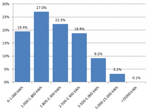
Figure 1. Consumption distribution for domestic residents in 2019 (elaboration from [3]. Only “protected” contracts)
As far as the electricity consumption distribution is concerned, about 46% of the residents consume less than 1800 kWh/y, corresponding to 24% of the total resident consumption. As can be deduced from Figure 1, 68.1% of the Italian users have annual consumptions higher than 1,000 and lower than 3,500 kWh/y.
2.2 Representativeness of the group under investigation
The electricity consumption can be very different from user to user, depending on the composition of the family, the daily habits and other variables, such as the day of the week, the hour of the day and the season.
The group under investigation involves 10 employees working with typical office equipment.
Since the group is small, its representativeness has been investigated. They belong to 10 different families, formed, in average, by 2.2 members. This is very close to the number of the Italian average value of 2.3 already mentioned in the previous section.
The electricity consumption of a single house is not simply proportional to the number of components and, moreover, the group under investigation, involving family consumptions, inevitably averages and compares, on one side (in the office building) employee consumptions and, on the other side (in the households), an average of different consumption styles, including children and cohabitants. Since this study is focused on the average behavior, all the consumptions will be normalized to the number of members, assuming the variability is cancelled out in the average.
In the group analyzed here, 80% of the families have consumptions between 1,000 and 3,500 kWh/y, with a peak in the interval [1000:1800]. Therefore, the 10 families under investigation has a consumption distribution not far from that of the whole Italian population (Figure 1). The annual mean electrical consumption of the sample families turns out to be 2,080 kWh/y/location, that is very close to the value 2,184 kWh/y/location, as reported in Table 2.
The representativeness of the typical hourly load curve [4] is checked with a comparison with [5], describing the Italian average electric hourly load curve for households (average variation behavior during the day). This includes the values of 396 houses, sampled in 2011 in the whole Italian territory. The peaks of 500 W are at the hours 20-21 and the minima (150 W) at 4-5 (a.m.) during both the weekdays (i.e. from Monday to Friday included) and the weekend (Figure 2). In the sample of [5], the annual mean electricity consumption is 2,637 kWh/y/location and the average value of the components in a family is 2.7.
Figure 2. Load curve during the day [5]
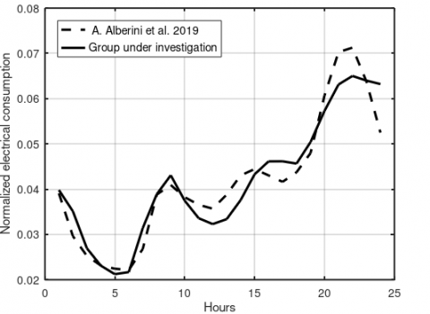
The average electric hourly load curve of the household for the group under investigation has been calculated averaging the data of the 10 resident families during the weekdays and applying a moving average of three samples to smooth the shape. Normalizing the data to the annual consumption, and comparing them to [5], the arising curves turn out very close (Figure 3).
It can be concluded that, even if the chosen group of families is quite small (10 families), this can be approximately be considered representative of the Italian average family, having similar values for the number of components, the average load curve and the distribution of the annual electric consumption.
As far as the average electricity consumption of the employees at the office building is concerned, it has been obtained averaging the behavior of more than 70 people and it has been verified by a comparison with the results obtained in an identical building. This is a number considered to be statistically representative for the scope of this study.
Figure 3. Sample representativeness of the load curve
3.1 Description and method
The people of the sample under investigation work in the same building (in Bologna, Italy) as employees, using typical office equipment, with R&D and administrative tasks. Electric consumption is not monitored individually, but the data refer to the whole building, hosting, in about 70 rooms and 1600 m2, about 100 employees (with an average of 75 employees really present daily).
The monitored data are collected in the years 2018-2020, separately, according to three different uses: lighting (annual contribution of 16%), air conditioning (17%) and Power supply at the Sockets (P.S.) (for PCs, servers, monitors, printers, drivers, copy machines, etc.) (contribution of 67%). The average contribution due to air conditioning, in July and August, turns out to be about 40-50%.
A software has been developed for the data monitoring and analysis: the data are collected using the Apache Camel routing and mediation engine, with a custom and internally developed Modbus connector. These components are deployed in a deep customized Apache Karaf container, named SignalMix. PostgresSQL has been used as DataBase Management System tier, and Java for introspection and data analysis.
The average quarter-hour electrical load curve was calculated adding the three electrical components (lighting, air conditioning and P.S.) and applying a spline interpolation to achieve a continuous load curve in case of lack of data for less than 6 hours.
Table 3 shows the number of PCs and of monitors per employee. The number of electronic devices per employee turns out to be about 4.
The annual electricity consumption for the building turns out to be about 52,268 kWh.
Since the total electric consumption of the buildings obviously depends on the number of people actually present at work, an evaluation of the building occupancy is necessary, as studied also in [6]. The number of people nominally employed in the staff, has not been considered a value precise enough, since the absence due to many factors (e.g. smart working, tasks outside the building, flexible timetables, holidays) make unpredictable, on daily basis, the number of people really present in the building.
Therefore, an algorithm has been developed in order to evaluate, in real time, the actual occupancy of the building, by monitoring and recording (anonymously) when each person enters and exits.
Table 3. PC and monitors normalized to the number of employees (87 in staff)
|
|
Devices per employee |
|
PC/employee |
1.28 |
|
Monitor/employee |
1.34 |
|
Number of employees per office |
1.24 |
|
Total devices (PCs, monitors, printers, etc.) |
4.0 |
In this way, the electric load and the consumption, day by day, can be normalized to the actual number of employees in the building and an average value per employee can be estimated. Only normalized values can be somehow useful in evaluating the energy efficiency of the devices and of the behaviors and in planning interventions to improve them. This methodology becomes particularly interesting when smart working becomes an important time fraction of the job, as happened in many months of the years 2020-21.
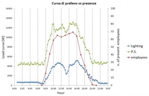
In order to visualize the correlation between occupancy and power load, both of these quantities are displayed in the same chart in Figure 4: the loads due to lighting and to P.S. are separated during a typical working day. It is clear how the load increases with higher occupancies and how it decreases during lunch time.
Figure 4. Power load vs building occupancy
In this way, it is possible to easily separate the contribution due to the base load (independent of the occupancy) from the contribution due to the presence and work in the office.
With this approach, the building occupancy has been calculated as integration in time of the number of people: Occupancy =$\left(\sum_{i} p\left(t_{i}\right) \cdot \Delta t_{i}\right)$, where p(ti) denotes the number of people present in the building at time ti and ti the time of presence of p(ti) people.
The average load per employee can thus be obtained by subtracting from the total daily consumption [kWhd], the base load kWb times 24h (obtaining therefore the consumption due to all the employees) and dividing then by the occupancy of the day (people·hour):
$\frac{W}{\text { employee }}=\frac{\left[k W h_{d}-24 \cdot k W_{b}\right]}{\left(\sum_{i} p\left(t_{i}\right) \cdot \Delta t_{i}\right)}$ (1)
The value of kWb is assumed to be constant during the whole day.
The base load due to the P.S. varies in the range 2.1 kW (min) – 4.2 kW (max), with an average of about 3.2 kW. The variability of the base load is mainly due to the use of several servers. Normalizing to the number of employees, the P.S. base load turns out to be 36 W/employee on average. The contribution of the base load is high: the base load for the P.S. weighs about 45-50% on the total P.S. consumption and the percentage of the consumption out of the working time (from 9 p.m. to 7 a.m. and during weekends and holidays), summing up all the components, turns out to be 35% on the total consumption.
The power load, averaged per employee (job in presence), summing up P.S. and lighting (without considering air conditioning), turns out to be about 100-110 W/employee in July and about 200-230 W/employee in December (2018). The motivation of this season dependency is due to the use of heating and lighting devices.
All these contributions drive a daily electric consumption per employee, considering 365 days and the actual presence of the employees in the office, of 2.2 [kWh/day/person]. When excluding air conditioning and the base load, one can estimate that the consumption of the employee is 1-1.2 kWh/day/person. Obviously, these data refer to average values and high fluctuations are present due to the heterogeneity of the electronic devices, job tasks of the employees, day of the week, external conditions of illumination and temperature.
3.2 Variation in the lockdown periods
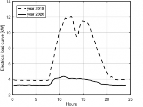
The average quarter-hour electrical load curve of the 2020 “strict lockdown” period (16 March-17 May) has been analyzed and compared to that of the previous year. Figure 5 shows the downfall of the average values throughout the day due to the absence of most of the employees, leaving almost only the base load consumption.
Table 4. Electricity consumption change in the offices
|
|
kWh/d/p 2019 |
kWh/d/p 2020 |
Changes in kWh/d/p |
|
From March 16 to May 17 |
2.14 |
1.13 |
- 1.01 (- 47 %) |
Note: d = day and p = person.
The average values of the electricity consumption in the building during the 2020 “strict lockdown” was investigated as well: the results, normalized per day (d) and person (p), are reported in Table 4. The consumption turns out to be lower by about 47% and the value of variation (1.01 kWh/d/p), is consistent with the value obtained in the previous section, referring to the consumption without air conditioning and the base load (1-1.2 kWh/d/p).
Figure 5. Variation of the average electrical load curve in the office buildings during weekdays (“strict lockdown” period)
4.1 Description and methods
The data of the electric consumption in the houses are retrieved directly by the residents themselves thanks to the recent platform developed by ARERA (the Italian authority for the energy) [7]. This service allows every Italian household owner to monitor some KPI data and to download his own data composed of quarter-hour electricity time series (consumption curves and related average load curves).
The raw data related to the group under investigation concerns the employees and their family members (10 POD) starting from March 1, 2019.
The electric load curves have been analyzed during the first “strict” lockdown, after and some months later than the first lockdown restrictions. These 3 periods are labelled respectively as “strict”, “partial”, “post” lockdowns, as reported in Table 5, where the exact dates are shown. All the 3 periods refer to 45 working weekdays. The load curves of the 2020 data periods considered for the 10 families have been compared with respect to the same periods of 2019, in order to avoid the influence of seasonality.
Table 5. Schedule of the analysis
|
Label of the lockdown measures in 2020 |
From |
To |
Available dataset |
|
Strict |
March 16 |
May 17 |
10 household and related office building |
|
Partial |
May 18 |
July 20 |
10 household |
|
Post |
Sept. 15 |
Nov. 17 |
10 household |
The analysis was performed including only the weekdays for each period in order to evaluate the electrical consumption at different levels of mobility restrictions and smart working adoption. The average electrical load curve of the households was calculated by simply averaging the electric load curve of the 10 resident families. A moving average over a sliding window of five elements has then been applied to smooth the shape of the resulting load curve.
4.2 Variation in the lockdown periods
The electricity consumption in kWh for each period, the average values per person and the respective variations from 2019 to 2020 (in absolute and in percentage) are reported in Table 6.
The average electrical load curves for each period in 2019 and in 2020 are plotted in Figure 6, 7 and 8, showing the average excesses and reductions in the electricity demand throughout the day.
Table 6. Domestic electricity consumption changes
|
Lockdown period |
kWh/d/p 2019 |
kWh/d/p 2020 |
Changes in kWh/d/p |
|
Strict |
2.25 |
3.40 |
+ 1.15 (+ 51 %) |
|
Partial |
2.52 |
3.05 |
+ 0.53 (+21 %) |
|
Post |
2.67 |
2.67 |
= |
Note: d = day and p = person.
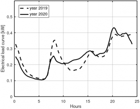
Figure 6. Variation of the domestic electrical load curve during weekdays (“strict” lockdown period)
Figure 7. Variation of the domestic electrical load curve during weekdays (“partial” lockdown period)
Figure 8. Variation of the domestic electrical load curve during weekdays (“post” lockdown period)
5.1 Description and methods
In this section PV panels are supposed to be installed, without energy storage, over the building where people work and over the homes of the people under investigation. This hypothesis is useful to evaluate the impact of lockdown and smart-working on PV self-consumption and PV self-sufficiency in this case study, as an example of tertiary and domestic sector.
The maximization of self-consumption and self-sufficiency represents a common goal to increase energy independency, to lower the stress on the electricity distribution grid and to reduce the dimension and losses of a possible storage [8].
In this study, PV self-consumption (kWh) (also called absolute self-consumption [8]), refers to the consumption of self-produced energy (i.e., the minimum between load and production), while the PV self-consumption rate refers to the ratio between PV self-consumption and the total PV production. On the other side, the PV self-sufficiency rate refers to the ratio between PV self-consumption and the total consumption.
The results are obtained simulating, hour by hour, the PV production, following method [9], according to real solar radiation data of 2019 [10] and assuming system losses of 10%. The nominal PV power (kWp) has been chosen in such a way that the PV annual production (in kWh) is equal to the annual consumption (of the office building or of the average behavior of homes). This criterion, detached from other economical choices, is useful to analyze and compare the two situations (home and work). The PV nominal powers thus turn out to be:
The location of the panels has been chosen in Bologna (Italy), with 30° of tilt, south direction. The data analysis was performed for all the days of the week (not only workdays). Figure 9 shows some days of example for the electrical load, PV production and PV self-consumption curves in the office and in household. As expected, during the night, consumption is higher than production. The reverse happens during the daytime, where production is much higher than consumption.
Figure 9. Week example of load (black), PV production (red) and PV self-consumption (blue) curves in 2019
5.2 Variation in the lockdown periods
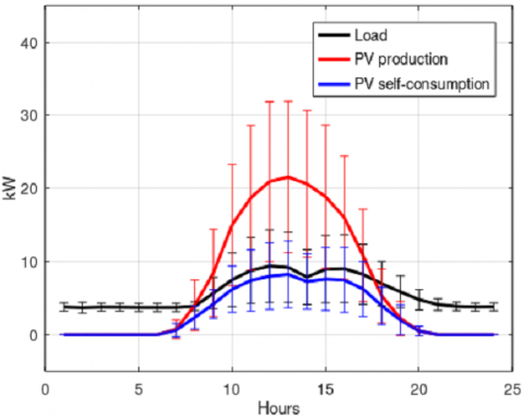
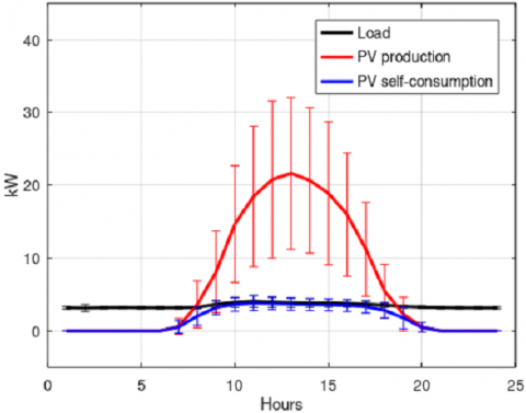
The load curve average behavior during the day, of the PV production and of the self-consumption, for the offices building, during March-May 2019 and during March-May 2020 (“strict lockdown” period of Table 5), is shown in Figure 10 and Figure 11 respectively.
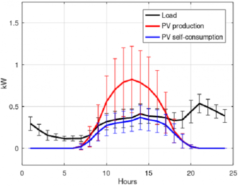
The same comparison was made for the households in Figure 12 and Figure 13.
In these figures the self-consumption curve appears a bit lower than the load curve during PV production because the charts represent an average with different levels of PV production (sunny and cloudy days).
Figure 10. Average curves in offices without lockdown
Figure 11. Average curves in offices with strict lockdown
Figure 12. Average curves in households without lockdown
Figure 13. Average curves in households with strict lockdown
The self-consumption computed over 56 days in the March-May period (excluding some incomplete days with respect to 63 total days) turns out to be 4,031 kWh in 2019 and 2,228 kWh in 2020 for office building, whereas it turns out to be 112 kWh in 2019 and 175 kWh in 2020 for the average household.
Table 7. Self-consumption without and with lockdown
|
Lockdown period (16/03-17/05) |
kWh/d/p 2019 |
kWh/d/p 2020 |
Changes kWh/d/p |
|
Office building |
0.96 |
0.53 |
- 0.43 |
|
Household |
0.91 |
1.42 |
+ 0.51 |
Note: d = day and p = person.
Table 8. Self-consumption rate without and with lockdown
|
Lockdown period (16/03-17/05) |
Self-cons. rate 2019 |
Self-cons. rate 2020 |
Changes |
|
Office building |
44.0% |
24.4% |
- 19.6 points |
|
Household |
32.1% |
50.4% |
+ 18.3 points |
Table 9. Self-sufficiency rate without and with lockdown
|
Lockdown period (16/03-17/05) |
Self-suff. rate 2019 |
Self-suff. rate 2020 |
Changes |
|
Office building |
52.3% |
48.1% |
- 4.2 points |
|
Household |
39.6% |
41.8% |
+ 2.2 points |
Table 7 and Table 8 show the results, respectively in normalized and percentage values, for the PV self-consumption, whereas the Table 9 shows the results, in percentage values, for the PV self-sufficiency.
The electricity consumption at the office building in the 2020 “strict lockdown” dropped down compared to the corresponding periods in 2019: it changed from 2.1 to 1.1 kWh/d/p (Table 4).
Electricity consumption of households during and immediately after the 2020 lockdown is, as expected, higher than the corresponding periods in 2019. It changes from 2.3 to 3.4 kWh/d/p, with an increase of about 51% during the 2020 lockdown (with respect to the same period in 2019) and it remains higher of about 21% in the “partial” lockdown period (Table 6).
The average increase at the households (+1.15 kWh/d/p) is consistent with both the corresponding decrease at the office (-1.01 kWh/d/p). Moreover, the latter is aligned with the estimated consumption at the office, without air conditioning and the base load (1-1.2 kWh/d/p).
In the “post lockdown” period, when the main restrictions have been removed and the occupancy within offices rises again, the electricity consumption in the households in 2020 is close to the 2019 value (Table 6).
The domestic electrical load curve during weekdays in the “strict lockdown” period appears higher from about 9:00 to 24:00 due to the presence of people at home, in smart working, distance learning and other home activities (Figure 6). About 60% of the increase of the daily average consumption appears in the hours 8-18 and about 42% becomes self-consumption.
The increase of the electrical load curve (with respect to the previous year) continues with less intensity in the “partial lockdown” period.
In general, in order to maximize self-consumption, since job is usually practiced during daylight hours, it is ideal to place PV production at the workplace: PV installations are usually more appropriate at the offices, because production tends to be higher (higher solar radiation) when the power load is higher (daylight working hours).
At the office building, in the case analyzed, even without smart working, self-consumption and self-sufficiency rates are not that high (44% and 52%) because of high contribution of the base load: 35% of the contribution to the total consumptions occurs overnight (from 9 p.m. to 7 a.m.) (see tails in Figure 10).
Smart working shifts consumption towards the houses: self-consumption at the office building drops from 44% to 24% (the numerator decreases; see Figure 11). Self-sufficiency, on the other hand, changes only from 52% to 48% since both self-consumption and total consumption (numerator and denominator) drop in the same area (see again Figure 11).
Concerning consumption at home, self-consumption started from a lower value (32%) than the self-consumption at the offices (44%), since most of the people, during the day (when the radiation is higher), stay out of home. Smart-working has a positive impact in PV at home because, increasing the balance of the consumptions during the day, makes the load curve closer to the production curve. Self-consumption in this way acquires values slightly higher than that of the office before smart working (50% vs 44%).
In order to obtain higher values of self-consumption it would be necessary to decrease the base load in both the building offices and in the households and to decrease the nominal power of the PV installed.
In smart working, in the case study here analyzed, every person shifts, from the office to home, about 1.0-1.2 kWh/day. This consumption concerns mainly typical office equipment, electronic devices and lighting, but also some no-working related consumptions (family components at home). At the office building remains the base load, which in the case analyzed, turns out to be 0.8 kWh/d/p.
With the approximations with which we worked, no variation of the total electric consumption has emerged. Of course, the main advantage of smart working remains the energy saving in transport to move from home to the workplace.
These results have been obtained thanks to a methodology developed to estimate the actual office building occupancy, based on recording the transit of people at the building entrance. This approach becomes particularly interesting when smart working increases and therefore the building occupancy is difficult to estimate a priori.
Since the “shifts” are concentrated during the working hours, which are daylight hours, this impacts on PV self-consumption of supposed PV panels installed at the office building and at home. In the case analyzed, and assuming the nominal power kWp such that PV annual production is equal to annual consumption, homes do not have high values for the self-consumption (32%). This is due to the fact that most of the people work outside home during the day. With “full” smart working, self-consumption acquires values slightly higher than that of the office building without smart working (50%). About 42% of the increase of the household total consumption becomes self-consumption.
In the office building, self-consumption drops from 44% to 24%, while self-sufficiency remains at a level of about 50%.
In the next years, with “soft” smart working, a value between these two extremes could be envisaged. These results are, on the other hand, dependent on the chosen PV nominal powers and need to be generalized.
Future investigations will involve also the extension of the study to the whole year, a wider sample of people, and a quantification of the economic variables.
Financial support for this work has been provided by Project 1.7 “Technologies for the efficient penetration of the electric vector in the final uses” within the “Electrical System Research” Program Agreements 19-21 between ENEA and the Ministry of Economic Development.
Authors thank Mirco Galigani and Salvatore Giordano for the help in the development methods to monitor building occupancies.
|
d |
day |
|
kWp |
kilowatt-peak |
|
p |
person |
|
POD |
Point Of Delivery |
|
PV |
Photovoltaic |
|
P.S. |
Power supply at the Sockets |
|
y |
year |
[1] Consumi 2019, Terna, 2020. Available: https://www.terna.it/it/sistema-elettrico/statistiche/pubblicazioni-statistiche.
[2] Annuario statistico 2019, ISTAT, 2019. Available: https://www.istat.it/it/archivio/236772.
[3] Relazione annuale – Stato dei servizi 2019 - volume I, ARERA, 2020. Available: https://www.arera.it/allegati/relaz_ann/20/RA20_volume1.pdf.
[4] Price, P. (2010). Methods for analyzing electric load shape and its variability (No. LBNL-3713E). Lawrence Berkeley National Lab. (LBNL), Berkeley, CA (United States). https://doi.org/10.2172/985909
[5] Alberini, A., Prettico, G., Shen, C., Torriti, J. (2019). Hot weather and residential hourly electricity demand in Italy. Energy, 177: 44-56. https://doi.org/10.1016/j.energy.2019.04.051
[6] Kim, Y.S., Srebric, J. (2017). Impact of occupancy rates on the building electricity consumption in commercial buildings. Energy and Buildings, 138: 591-600. https://doi.org/10.1016/j.enbuild.2016.12.056
[7] Il Portale Consumi, ARERA, https://www.arera.it/it/consumatori/portaleconsumi.htm.
[8] Luthander, R., Widén, J., Nilsson, D., Palm, J. (2015). Photovoltaic self-consumption in buildings: A review. Applied Energy, 142: 80-94. https://doi.org/10.1016/j.apenergy.2014.12.028
[9] Di Cristofalo, S. (2016). ProgettoCNR Energy+: metodo di calcolo semplificato per la scomposizione della radiazione solare globale e la stima della produzione da fotovoltaico. http://eprints.bice.rm.cnr.it/14398/.
[10] Manuale Dext3r, ARPAE. Available: https://simc.arpae.it/dext3r/doc/GuidaDext3r.html.