Pamela Vocale* | Matteo Malavasi | Luca Cattani | Fabio Bozzoli | Sara Rainieri
OPEN ACCESS
To assess the performance of triple tube heat exchangers, it is not possible to apply the traditional methods (e.g., Wilson plot method) because they can be only applied to the classical shell-in-tube configuration that can be easily modelled by the logarithmic mean temperature difference approach. Therefore, to overcome this limitation, some new methodologies have been proposed in the literature and, among them, a promising tool is represented by the parameter estimation procedure. Parameter estimation procedure is a powerful technique already adopted in many engineering applications. However, this procedure requires, for the application investigated in the present study, a detailed numerical model of the triple tube heat exchanger and the measurement of the temperature of the fluids in each tube at inlet and outlet sections. These elements make its application feasible only in well-equipped research labs, limiting its massive employment in industrial facilities. In this paper, a novel parameter estimation procedure to characterize the thermal behavior of the triple concentric-tube heat exchanger is proposed. This approach is based on a simple model of the exchanger and it requires to measure the fluid temperature only in four sections. The simplified proposed procedure is numerically validated and compared to the full one.
triple tube heat exchangers, parameter estimation, Nusselt number correlation
Heat exchangers play a major role in a wide range of thermal processes in both the residential and industrial sectors, such as in air conditioning, food treatment, and electronic cooling. Although the design and operation of these devices have been studied for a long time, the heat transfer enhancement of heat exchangers represents a key technological challenge because of rising cost of energy and raw materials.
A promising technology, widely used in food and pharmaceutical industries, is represented by the triple concentric-tube heat exchangers (TTHE), in which the heat transfer is enhanced in comparison with the double tube heat exchangers, due to the additional passage that improves the heat transfer and provides a larger surface area for the heat transfer per unit length.
Despite the advantages and the wide use of TTHEs, only few studies investigated heat transfer phenomena in this kind of device, as highlighted by Kumar and Hariprasath in their recent review [1].
Computation of overall heat transfer coefficients in a TTHE is more complicated respect to the cases of double tube or shell and tubes heat exchanger because the two overall heat transfer coefficients (at both sides of the annulus) are not independent of each other, making it necessary to solve them simultaneously.
Batmaz and Sandeep [2] and Radulescu et al. [3] proposed and developed a procedure that included a calculation algorithm able to determine the overall heat transfer coefficients and axial temperature distribution in a TTHE.
Gomaa et al. [4] evaluated the heat transfer coefficient of the inner annulus, by introducing an average log-mean temperature difference between the three fluids, which was defined as the arithmetic mean between the log-mean temperature difference between the fluid in the annulus and the one in the external tube and the log-mean temperature difference between annulus and internal pipe. The same approach was adopted by Tiwari et al. [5].
Ünal [6, 7] developed closed form expressions for the effectiveness-NTU relations, including both the counter-flow and parallel flow configurations.
However, it is difficult to generalize the data available in the literature to TTHEs, due to the specificity of each product, thermal treatment and geometrical configuration, making the thermal design of these apparatuses critical and requiring the measurement of the thermal performances.
One of the simplest methods used to estimate the inside heat transfer coefficient in heat exchangers is the Wilson plot technique [8]. By adopting this approach, the internal heat transfer coefficient can be indirectly evaluated from the experimental measurements of the overall thermal resistance. Since the technique proposed by Wilson presented some limitations for the application in TTHEs (e.g., impossibility to define a univocal behavior of the “shell” side), several different approaches have been proposed in the literature to overcome these limits [9]. Among these techniques, a promising tool is represented by the parameter estimation procedure.
Parameter estimation procedure is a powerful technique already employed for numerous engineering applications and demonstrates to work satisfactorily on many different types of heat exchanger geometry [10-14]. However, this procedure usually requires a detailed numerical model of the triple tube heat exchanger and the measurement of the temperature of the fluids at six tube inlet and outlet sections. This kind of measurement is not easily implementable because most of TTHE uses only two fluids which have only one inlet and one outlet section. These requirements make the application of the classical function estimation approach feasible only in well-equipped research labs, limiting its massive employment in industrial facilities.
In this paper, a novel parameter estimation procedure that enables to characterize the thermal behavior of the triple concentric-tube heat exchanger is presented. This procedure, validated by means of synthetic data, is based on a simplified model of the exchanger and it requires the measurement of the temperature of the fluids at only four sections.
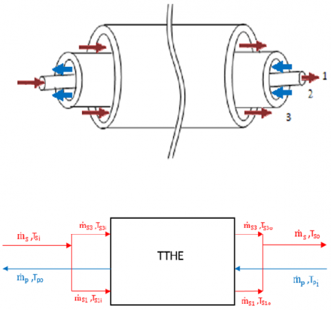
TTHE investigated in the present study operates in a counterflow arrangement, which is the most commonly adopted in industrial applications since it provides the best performance. In this configuration, the process fluid to be heated flows into section 2 (Figures 1), and the hot service fluid flows both in sections 1 and 3.
From a practical point of view, the service fluids that flow in the inner tube and in the outer annular section come from a single source, in fact they have the same temperature when they enter the heat exchanger.
At the outlet of the heat exchanger, however, the situation is quite different: the service fluids have different temperatures due to the different flow rates and heat transfer surfaces of the sections involved.
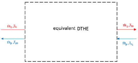
In the present paper it is proposed a simplified model of the physical problem that is considered as an equivalent Double Tube Heat Exchanger (DTHE) in counter-flow arrangement, as schematized in Figure 2, where the red lines indicate the service side, while the blue ones the product side.
Figure 1. Investigated TTHE. a) 3D model; b) schematic representation
The geometrical properties of the equivalent DTHE were derived from the characteristics of the TTHE. In particular, the arithmetic means between the hydraulic diameters of the two service sections of the TTHE (i.e. sections 1 and 3 in Figure 1) was assumed as diameter of the service side, while the diameter of the product side was assumed equal to the hydraulic diameter of the inner annulus of the TTHE (i.e. section 2 in Figure 1). Moreover, the equivalent DTHE was characterized by the same heat transfer areas of the TTHE.
Figure 2. Sketch of the equivalent DTHE
By assuming that the steady state condition was verified and that the heat exchanger was perfectly thermally insulated from the environment and the heat conduction in the flow direction was negligible, the average overall heat transfer coefficient U for the inner heat transfer surface area Ai could be obtained from the equation:
$U=\frac{Q}{A_{i} \Delta T_{m l}}$ (1)
where, ∆Tml was the logarithmic mean temperature difference and Q was the heat transfer rate exchanged, which could be obtained from the energy balance for both the process and the hot service fluids.
By assuming that both the process and the hot service fluids were single phase, incompressible, and with constant thermal properties, the heat transfer rate exchanged was evaluated as follows:
$Q=\dot{m}_{p} c_{p p}\left(T_{p, \text { out }}-T_{p, \text { in }}\right)$ (2)
$Q=\dot{m}_{s} c_{p s}\left(T_{s, \text { in }}-T_{s, \text { out }}\right)$ (3)
where, $\dot{m}$ was the mass flow rate, T was the fluid bulk temperature and cp were the fluid specific heat at a constant pressure.
The subscripts p and s indicated the product and the service fluid, and the subscripts in and out referred to the corresponding inlet and outlet conditions.
The inlet temperatures of both process and hot service fluids ($T_{s, \text { in }}$ and $T_{p, \text { in }}$) were assumed to be known, and so were the two mass flow rates ($m_{s}$ and $m_{p}$).
The overall heat transfer coefficient was related to the product and service fluid convective heat transfer coefficients by the following equation:
$\frac{1}{U A_{i}}=\frac{1}{h_{i} A_{i}}+R_{w, e q}+\frac{1}{h_{e} A_{e}}$ (4)
where, hi and he indicated the convective heat transfer coefficients, respectively, Ae was the external heat exchanger surface area and Rw,eq is the thermal resistance of the wall.
Since in the TTHE there were two thermal resistances in parallel configuration (i.e. one due to wall that separates sections 1 and 2 and one due to wall that separates sections 2 and 3), the wall thermal resistance for the equivalent DTHE was evaluated by considering the equivalent thermal resistance, as follows:
$R_{w, e q}=\frac{R_{w 12} \quad \cdot \quad R_{w 23}}{R_{w 12} \quad +\quad R_{w 23}}$ (5)
The wall thermal resistance for each wall was approximated as reported in [15]:
$R_{w}=\frac{\ln \left(D_{o} / D_{i}\right)}{2 \pi \lambda_{w L}}$ (6)
where, Di and Do were the internal and external diameter of the pipe, respectively, $k_{w}$ and L were the wall thermal conductivity and the pipe length, respectively.
The convective heat transfer coefficients were evaluated by the Nusselt numbers, which were expressed by the following equations:
$N u_{p}=\frac{h_{p} D_{h p}}{\lambda_{p}}$ (7)
$N u_{s}=\frac{h_{s} D_{h s}}{\lambda_{s}}$ (8)
where, Dh was the hydraulic diameter and λ was the fluid thermal conductivity.
The Nusselt numbers in the fully developed region were expressed as a function of Reynolds and Prandtl numbers [15]:
$N u_{p}=C_{p} R e_{p}^{\alpha_{p}} P r_{p}^{\beta p}$ (9)
$N u_{s}=C_{S} R e_{s}^{\alpha_{s}} P r_{s}^{\beta_{s}}$ (10)
where, C, α, β were a set of characteristic coefficients of each of the two sections of the heat exchanger under test.
Substituting Eqns. (9) and (10) in Eq. (4), U was obtained by:
$U=\frac{1}{A_{i}}\left(\frac{D_{h p}}{A_{i} \lambda_{p} C_{p} R e_{p}^{\alpha_{p}} P r_{p}^{\beta_{p}}}+R_{w}+\frac{D_{h s}}{A_{e} \lambda_{s} C_{s} R e_{s}^{\alpha_{s}} P r_{s}^{\beta_{s}}}\right)-1$ (11)
To identify the outlet temperatures $T_{p, o u t}$ and $T_{s, \text { out }}$ the concept of the log means temperature difference, ΔTml, which was applied to the counter-flow configuration, was used [15].
$\Delta T_{m l}=\frac{\Delta T_{2}-\Delta T_{1}}{\ln \left(\Delta T_{2} / \Delta T_{1}\right)}$ (12)
where, $\Delta T_{1}$ and $\Delta T_{2}$ were evaluated as follows:
$\Delta T_{1}=T_{s, \text { in }}-T_{p, \text { out }}, \quad \Delta T_{2}=T_{s, \text { out }}-T_{p, \text { in }}$ (13)
Substituting Eqs. (2), (3) and (13) in Eq. (1) yields the following:
$Q=(B-1)\left[\frac{T_{s i}-T_{p i}}{\left(\frac{B}{\dot{m}_{p} c_{p p}}-\frac{1}{\dot{m}_{s} c_{p s}}\right)}\right]$ (14)
where, B is defined as follows [14]:
$B=\exp \left[U A_{i} \frac{\left(\dot{m}_{s} c_{p s}-\dot{m}_{p} c_{p p}\right)}{\dot{m}_{s} c_{p s} \cdot \dot{m}_{p} c_{p p}}\right]$ (15)
The outlet temperatures for both the product and the service fluids were obtained as follows:
$T_{p, o u t}=T_{p, i n}+\frac{Q}{\dot{m}_{p} c_{p p}}$ (16)
$T_{s, o u t}=T_{s, i n}-\frac{Q}{\dot{m}_{s} c_{p s}}$ (17)
Eqns. (16-17) represent the direct formulation of the problem under study that is concerned with the determination of the outlet temperatures of the two modelled sections when all the coefficients C, α, β are known. In the inverse formulation, the coefficients C, α, β are instead regarded as being unknown, whereas the outlet temperatures of the two modelled sections are measured.
In the inverse formulation, the values of the outlet temperatures, computed by solving the direct problem (Eqns. (16-17)) are forced to match the experimental temperature values, by tuning the coefficients C, α, β. The matching of the two temperature distributions (the computed and the experimentally acquired) could be easily performed under a least square approach. Therefore, the coefficients C, α, β could be estimated by minimizing the following functional:
$S(\boldsymbol{P})=\sum_{j=1}^{N}\left[\boldsymbol{T}_{\text {exp }, j}-\boldsymbol{T}_{\text {pred }, j}\right]^{2}$ (18)
where, P was the vector of the parameters that have to be estimated, Texp and Tpred were the measurements vector and the predicted temperatures vector, respectively, and N was the total number of measurements.
The measurements vector was composed as follows:
$\boldsymbol{T}_{\text {exp }}=\left[\boldsymbol{T}_{p, \text { out }}, \boldsymbol{T}_{s, \text { out }}\right]$ (19)
Tp,outand Ts,out were the outlet temperatures of the both product and service sides measured for the N tests.
Analogously the vector Tpred included the temperature values obtained by solving the full direct problem presented in [16].
In the most general case, for the TTHE all the six parameters (the C, α, and β coefficients for both the product and the equivalent service side had to be estimated.
As the problem was non-linear with respect to the unknown variables, a non-linear optimization algorithm was used. One of the most common algorithms utilized in an inverse problem approach is the non-linear fit algorithm based on the iterative reweighted least squares method [14].
To express the reliability of the parameter estimates and to compare the relative precision of different parameter estimates the 95% confidence interval, CI95%, and the coefficient of variation, CV, are generally used [17]. Regarding the parameter Pi, they are defined as follows:
$C I_{P_{i}}^{95 \%}=\left(P_{i}-1.96 \sigma_{P i}, P_{i}+1.96 \sigma_{P i}\right)$ (20)
$C V_{P i}=\frac{\sigma_{P i}}{P_{i}}$ (21)
The simplified model proposed in the present study was validated by means of synthetic data. The geometrical and thermal characterizations of TTHE and of the equivalent DTHE are reported in Tables 1 and 2.
Table 1. Geometrical characteristics of the investigated TTHE
|
Parameter |
Value |
|
Dh1 (m) |
0.0409 |
|
Dh2 (m) |
0.0186 |
|
Dh3 (m) |
0.0108 |
|
L (m) |
10.10 |
|
Ai1 (m2) |
1.2990 |
|
Ai2 (m2) |
2.1237 |
|
Ae1 (m2) |
1.5326 |
|
Ae2 (m2) |
2.3172 |
Table 2. Geometrical characteristics of the equivalent DTHE
|
Parameter |
Value |
|
Dhs (m) |
0.0259 |
|
Dhp (m) |
0.0186 |
|
L (m) |
10.10 |
|
Ai (m2) |
3.4227 |
|
Ae (m2) |
3.8498 |
Synthetic data were obtained by solving the full direct problem presented in [16], by assuming a highly viscous fluid food (i.e., fruit purees or concentrated juices) and water, for the product and the service sides, respectively.
Constant physical properties of the fluids were as follows: ρs= 1000 kg∙m-3, λs= 0.6 W∙m-1∙K-1, μP= 1∙10-3 Pa∙s, cps= 4180 J kg-1K-1, ρp = 1054 kg∙m-3, μP= 2.6∙10-1 Pa∙s, λp = 5.9 10-1 W∙m-1∙K-1 and cps= 3852 J kg-1K-1. The heat exchanger was supposed to work in turbulent regime for the service side (18∙103 < Res < 65∙103) while the product was considered in a laminar condition with Repranging between 5 and 500. In particular, 225 operating conditions were generated.
To simulate the presence of experimental noise, the synthetic data obtained from the solution of the full direct problem were deliberately spoiled by random noise [16].
Synthetic data were elaborated with the inverse estimation procedure based on the simplified model presented in this study.
It has to be highlighted that the constant physical properties of the fluids were considered, so the modeled heat transfer mechanism was not sensitive to Prandtl number changes, making the estimation of βp and βs impossible with the inverse problem approach. Therefore, only the parameters Cp, αp, Cs and αs had to be estimated, whereas βp and βs were considered known.
The estimated parameters for noise level equal to 0.05 K, which is a common noise level in this kind of applications and experimental setup [16] are reported in Table 3.
Table 3. Results of novel parameter estimation procedure
|
Unknow parameter |
Estimated parameter |
CI95% |
CV |
|
|
Cp |
0.025 |
0.024 |
0.025 |
0.60% |
|
αp |
0.807 |
0.804 |
0.811 |
0.24% |
|
Cs |
0.006 |
0.005 |
0.006 |
4.71% |
|
αs |
0.788 |
0.779 |
0.798 |
0.60% |
It can be observed that the confidence intervals and the CVs are very small confirming the efficacy of the novel estimation procedure for the considered application. The highest value of CV is 4.7% underlying the very good results achieved.
To provide better insight in the evaluation of the effectiveness of the simplified approach a residual analysis was performed by computing the average estimation error on the heat power exchanged, defined as follows:
$E_{Q}=\frac{[[ Q_{\text {restored }}-Q_{\text {exact }} \quad ]]_{2}}{[[ Q_{\text {exact }} \quad ]]_{2}}$ (22)
where, Qrestored and Qexact were the restored and exact heat power values, respectively.
The exact values of the exchanged heat power were considered the values employed in the full model [16] to generate the synthetic data, while the restored value was evaluated by adopting the simplified approach proposed in the present study.
The estimation errors on the exchanged heat power, evaluated by means of Eq. (22), for the values of the Reynold number of the service fluid considered in the present analysis are reported in Table 4. For each value of Res, the Reynold number of the product Rep varied in the range 5÷500.
It can be observed that although the estimation error changes depending on the value of Res, the maximum error was 2.09%, thus confirming the accuracy of the simplified model presented in this study.
Table 4. Estimation error on the exchanged heat power
|
Res |
EQ |
|
18’370 |
2.09% |
|
22’043 |
1.43% |
|
25’717 |
1.26% |
|
29’391 |
0.71% |
|
33’065 |
0.91% |
|
36’739 |
0.77% |
|
40’413 |
0.63% |
|
44’087 |
0.51% |
|
47’761 |
0.58% |
|
51’435 |
0.42% |
|
55’109 |
0.25% |
|
58’783 |
0.40% |
|
60’619 |
0.33% |
|
62’456 |
0.60% |
|
64’293 |
0.54% |
The average estimation error on the exchanged heat power Q, evaluated for the whole dataset was lower than 1%.
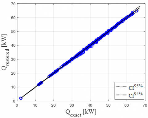
The restored values of the heat power for a noise level equal to 0.05 K against the exact ones are presented in Figure 3.
Figure 3. Comparison between exact and estimated heat power
It was found that the values of the exact heat power and the values obtained by adopting the outlet temperatures evaluated by applying the simplified model (Eqns. (16) and (17)) were in a very good agreement, as shown in Figure 3. In the same figure the confidence intervals are also depicted. They were evaluated by considering the standard deviation of the estimation error on the exchanged heat power, which, according to Eq. (22), was defined as follows:
$e_{Q}=\frac{Q_{\text {restored }}-Q_{\text {exact }}}{Q_{\text {exact }}}$ (23)
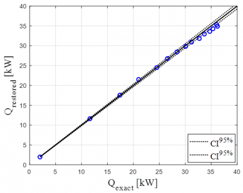
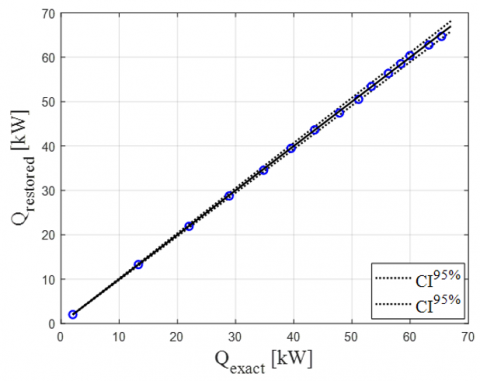
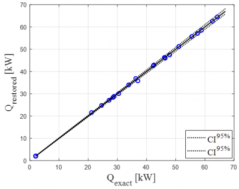
It was observed that the difference between the restored values of the heat power and the exact ones was dependent on the ratio between the values of the Reynold number of the product and service fluids. In particular, the highest difference was found for the lowest Res considered in the present study, while the lowest difference was found for the highest Resconsidered here.
These findings are confirmed by the graphs in Figures 4 and 5 where the restored values of the heat power for a noise level equal to 0.05 K are reported against the exact ones for a single value of Res, i.e. the minimum and the maximum investigated here.
Figure 4. Comparison between exact and estimated heat power for Res= 18’370
Figure 5. Comparison between exact and estimated heat power for Res= 64’293
It has to be highlighted that the results presented in Table 3 and in Figure 3 were obatined by considering a synthetic dataset composed of 225 data that implies in practical applications at least 225 experiments have to be performed.
To assess the feasibility of the simplified approach for practical applications a reduced dataset was considered. In particular, 25 operating conditions were investigated by keeping the same ranges of Rep and Res.
As expected by reducing the number of data, the parameter estimation procedure results in less accurate values, as demonstrated by the analysis of the coefficient of variation CV. In particular, the highest values of CV were 4.7% and 12.5% for the complete dataset and the reduced one, respectively.
The estimated parameters for the reduced dataset and for noise level equal to 0.05 K, are presented in Table 5.
Table 5. Results of novel parameter estimation procedure (reduced dataset)
|
Unknow parameter |
Estimated parameter |
IC |
CV |
|
|
Cp |
0.025 |
0.024 |
0.025 |
1.10% |
|
αp |
0.803 |
0.794 |
0.811 |
0.55% |
|
Cs |
0.006 |
0.005 |
0.008 |
12.53% |
|
αs |
0.785 |
0.760 |
0.810 |
1.64% |
Figure 6. Comparison between exact and estimated heat power (25 operating conditions)
However, it was found that the values of the exact heat power and the restored ones (i.e. obtained by applying the simplified model) were in a very good agreement even for reduced dataset, as shown in Figure 6 and in Table 6.
In particular, the maximum of the average estimation error on the heat power exchanged for the reduced dataset was comparable with the corresponding value obtained for the complete dataset, thus confirming the accuracy of the simplified model.
The application of the simplified approach to the reduced dataset confirms that the simplified model of the exchanger enables to properly evaluate the thermal performance of a TTHE. Moreover, the analysis presented here reveals that the simplified model requires only a very limited number of fluid temperatures.
Table 6. Estimation error on the exchanged heat power (25 operating conditions)
|
Res |
EQ |
|
18’370 |
2.17% |
|
29’391 |
1.08% |
|
44’087 |
0.43% |
|
58’783 |
0.46% |
|
64’293 |
0.61% |
The present work intends to propose a novel simplified approach for evaluating the thermal performance of a Triple Tube Heat Exchanger.
The validation of the proposed approach through synthetic data reveals that it is accurate and reliable. In particular, it allows to obtain an accurate evaluation of the heat power exchanged even when very limited data are available. This makes the proposed approach very suitable also for industrial application.
This work was partially supported by the Emilia-Romagna Region (Piano triennale alte competenze per la ricerca, il trasferimento tecnologico POR FSE 2014/2020).
|
A |
Heat transfer surface area, m2 |
|
C |
Multiplicative constant (Eq. (8)) |
|
CI95% |
Confidence interval |
|
CV |
Coefficient of variation |
|
cp |
Specific heat, J kg-1 K-1 |
|
D |
Diameter, m |
|
h |
Convective heat transfer coefficient, W m-2 K-1 |
|
L |
Heat exchanger’s length, m |
|
m ̇ |
Mass flowrate, kg s-1 |
|
Nu |
Nusselt number |
|
Pi |
Generic unknown parameter |
|
Pr |
Prandtl number |
|
Q |
Heat transfer rate, W |
|
Re |
Reynolds number |
|
Rw |
Wall thermal resistance, W K-1 |
|
Rw,eq |
Equivalent wall thermal resistance, W K-1 |
|
S |
Target function |
|
T |
Temperature, K |
|
U |
Overall heat transfer coefficient, W m-2 K-1 |
|
Greek symbols |
|
|
α |
Reynolds number exponent (Eq. (8)) |
|
λ |
Fluid thermal conductivity, W m-1 K-1 |
|
λw |
Wall thermal conductivity, W m-1 K-1 |
|
$\sigma$ |
Standard deviation |
|
Subscripts |
|
|
in |
Inlet section |
|
out |
Outlet section |
|
p |
Product |
|
s |
Service |
[1] Kumar, P.M., Hariprasath, V. (2020). A review on triple tube heat exchangers. Materials Today: Proceedings, 21: 584-587. https://doi.org/10.1016/j.matpr.2019.06.719
[2] Batmaz, E., Sandeep, K.P. (2008). Overall heat transfer coefficients and axial temperature distribution in a triple tube heat exchanger. Journal of Food Process Engineering, 31(2): 260-279. https://doi.org/10.1111/j.1745-4530.2007.00154.x
[3] Rădulescu, S., Negoiţă, L.I., Onuţu, I. (2016). Analysis of the heat transfer in double and triple concentric tube heat exchangers. In IOP Conference Series: Materials Science and Engineering, 147(1): 012148. https://doi.org/10.1088/1757-899X/147/1/012148.
[4] Gomaa, A., Halim, M.A., Elsaid, A.M. (2016). Experimental and numerical investigations of a triple concentric-tube heat exchanger. Applied Thermal Engineering, 99: 1303-1315. https://doi.org/10.1016/j.applthermaleng.2015.12.053
[5] Tiwari, A.K., Javed, S., Oztop, H.F., Said, Z., Pandya, N.S. (2021). Experimental and numerical investigation on the thermal performance of triple tube heat exchanger equipped with different inserts with WO3/water nanofluid under turbulent condition. International Journal of Thermal Sciences, 164: 106861. https://doi.org/10.1016/j.ijthermalsci.2021.106861
[6] Ünal, A. (1998). Theoretical analysis of triple concentric-tube heat exchangers Part 1: Mathematical Modelling. International Communications in Heat and Mass Transfer, 25(7): 949-958. https://doi.org/10.1016/S0735-1933(98)00086-4
[7] Unal, A. (2003). Effectiveness-NTU relations for triple concentric-tube heat exchangers. Int. Commun. Heat Mass., 30(2): 261-272. https://doi.org/10.1016/S0735-1933(03)00037-X
[8] Wilson, E.E. (1915). A basis for rational design of heat transfer apparatus. The J. Am. Soc. Mech. Engrs., 37: 546-551.
[9] Fernández-Seara, J., Uhía, F.J., Sieres, J., Campo, A. (2007). A general review of the Wilson plot method and its modifications to determine convection coefficients in heat exchange devices. Applied Thermal Engineering, 27(17-18): 2745-2757. https://doi.org/10.1016/j.applthermaleng.2007.04.004.
[10] Beck, J.V., Arnold, K.J. (1977). Parameter Estimation in Engineering and Science. James Beck.
[11] Orlande, H.R., Fudym, O., Maillet, D., Cotta, R.M. (2011). Thermal Measurements and Inverse Techniques. CRC Press.
[12] Luo, X., Yang, Z. (2017). A new approach for estimation of total heat exchange factor in reheating furnace by solving an inverse heat conduction problem. International Journal of Heat and Mass Transfer, 112: 1062-1071. http://dx.doi.org/10.1016/j.ijheatmasstransfer.2017.05.009.
[13] Rainieri, S., Bozzoli, F., Cattani, L., Vocale, P. (2014). Parameter estimation applied to the heat transfer characterisation of Scraped Surface Heat Exchangers for food applications. Journal of Food Engineering, 125: 147-156. https://doi.org/10.1016/j.jfoodeng.2013.10.031
[14] Vocale, P., Bozzoli, F., Mocerino, A., Navickaitė, K., Rainieri, S. (2020). Application of an improved parameter estimation approach to characterize enhanced heat exchangers. International Journal of Heat and Mass Transfer, 147: 118886. https://doi.org/10.1016/j.ijheatmasstransfer.2019.118886.
[15] Incropera, F.P., DeWitt, D.P., Bergman, T.L., Lavine A.S. (2007). Fundamentals of Heat and Mass Transfer. 6th ed. New York: John Wiley & Sons Inc.
[16] Malavasi, M., Cattani, L., Vocale, P., Bozzoli, F., Rainieri, S. (2021). Thermal characterisation of triple tube heat exchangers by parameter estimation approach. International Journal of Heat and Mass Transfer, 178: 121598. https://doi.org/10.1016/j.ijheatmasstransfer.2021.121598
[17] Blackwell, B., Beck, J.V. (2010). A technique for uncertainty analysis for inverse heat conduction problems. International Journal of Heat and Mass Transfer, 53(4): 753-759. https://doi.org/10.1016/j.ijheatmasstransfer.2009.10.014