Francesco S. Ciani* | Paolo Bonfiglio | Stefano Piva
OPEN ACCESS
Plumes fires are characterized by a turbulent nature with a large number of different scales. LES is used to solve the largest structures and to model the smallest ones. Grid size and time steps become decisive to place a limit between solved and modelled turbulence. A spectral analysis, both in frequency and wavenumber domain of the specific turbulent kinetic energy is an instrument to check for the information investigated. Unfortunately, the spectra in the wavenumber domain can be difficult to achieve adequately, because the specific turbulent kinetic energy values should be available in many points. This issue can be overcome by identifying a correlation law between frequencies and wavenumbers. An approach to identify this correlation law can be to adopt the IWC method. Here, for a test case of a turbulent reacting plume of burning propane, specific turbulent kinetic energy is analysed both in frequency and wavenumber and a correlation law between them is identified by using the IWC method. A study has been performed to evaluate the grid dependency of the specific turbulent kinetic energy spectra, by assessing the extension of the Kolmogorov power law region. The correlation results are discussed and compared with the Taylor’s hypothesis.
turbulence, fire, plume, CFD, IWC
The open source CFD code “Fire Dynamics Simulator” (FDS in the following) is widely used for the numerical modelling of fires in civil and industrial activities. A LES flow solver able to capture the time evolution of flame and smoke and their turbulent nature, characterizes the code. The LES approach allows us to solve the largest eddies and to model the smallest ones. The solved scale is proportional to the dimension of the grid cells and to the time intervals: the smaller they are, the smaller is the solved scale. This means that to solve highly turbulent flows and to show a significant number of turbulent structures, a large number of cells and of time steps is needed. It is therefore important to understand where the limit between resolved or modelled turbulence is placed. Significant information on this limit and its placement can be obtained with a spectral analysis of the turbulent kinetic energy of the flow.
The spectrum of a turbulent phenomenon can be studied in time and space domains. In the time domain, a frequency analysis is required, whereas in the space domain, a wavenumber analysis is required. For the natural time evolutionary behaviour of a turbulent flow, it is easy to produce the time steps required by the frequency analysis. On the contrary, the search for correlations in the wavenumber space is not practical, mainly due to the limited number of aligned and useful grid points.
This search becomes possible when a correlation between frequencies and wavenumbers is available. For this purpose, the most used approach is the Taylor's hypothesis [1], stating a linear dependency between frequencies and wavenumbers. This hypothesis has been extensively used, even if it is source of approximations [2].
As an example, we cite only the work of Comte-Bellot and Corrsin [3], who experimentally analyse a duct flow, where an approximation to isotropic turbulence is achieved with a regular grid. Following Taylor’s hypothesis, they calculate the spectrum of the specific turbulent kinetic energy in the wavenumber domain.
Taylor’s hypothesis is commonly applied by using the axial mean velocity to relate frequencies and wavenumbers. Unfortunately, in many situations it is difficult to identify a specific propagation velocity because the time averaged velocity can vary significantly in the space. In these situations, the identification of the correlation frequencies-wavenumbers can be difficult.
Recently, a more general approach is available in the literature, used especially for the analysis of acoustics and vibrations. A first approach, due to McDaniel and Shepard [4], is useful in finding, iteratively, a correlation between frequencies and wavenumbers. Berthaut et al. [5] generalise the method, named now Inhomogeneous wave correlation (IWC) method. The IWC method, starting from the spectra calculated in the frequency domain, allows us to obtain the so-called correlation law, i.e. a correlation between frequencies and wavenumbers. To the best Authors knowledge, an extension of the IWC method to turbulence has not yet been attempted.
Here, for a test case of turbulent reacting flow, the specific turbulent kinetic energy is analysed both in frequencies and wavenumbers domain; a correlation between frequencies and wavenumbers is found by using the IWC method.
The purpose of this study is thence to remark the correlations between grid spacing, time steps and solved scales of turbulence, through the spectra of the specific turbulent kinetic energy. Special care is given to the grid resolution; as the starting point the approach recommended by the FDS User Guide [6], consisting of a limitation of the ratio between the characteristic fire diameter and the grid size, is used.
As a result, the specific turbulent kinetic energy spectrum along the centreline of the fire plume is analysed to individuate the solved scales of the turbulent flow. Furthermore, it is verified whether the above-mentioned energy spectra exhibit the scaling laws in the inertial subrange by following the Kolmogorov theory. Furthermore, a grid refinement study is performed to evaluate the grid dependency of the turbulent kinetic energy spectra.
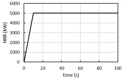
As the case study consideration is given to a turbulent plume fire in a 10 x 10 x 10 m cubic domain (Figure 1). The domain has a box shape with solid top and bottom surfaces. The lateral faces are free to communicate with the external ambient. A square burner (L = 1.5 m) is located in the centre of the bottom plane on a support 0.5 m height. Propane, released with such a flow rate as to achieve an imposed heat release rate (HRR), is used to fuel the fire. The HRR curve reaches, with a linear growth, a maximum value of 5 MW after 10 s (Figure 2).
The fire problem is addressed numerically using the CFD code FDS release 6.7.1, on a structured rectilinear grid. The case study is analysed on three uniform meshes (grid size 0.25 m, 0.125 m and 0.0625 m, respectively). Overall, grids of 64×103, 512×103 and 4096×103 nodes are generated. The starting grid is based on the practical rule proposed by the code FDS [6]. For all runs a time step of 10-3 s has been chosen, having always checked that the stability constraints are satisfied.
The bottom and top walls of the domain and the lateral surfaces of the burner are assumed to be non-participating. The remaining surfaces are modelled as openings.
LES with the Deardorff sub-grid model is used to perform the turbulence calculations.
Figure 1. Computational domain
Figure 2. HRR curve imposed to the burner
To the velocity components $\tilde{u}_{l}\left(x_{i}, t\right)$ along the centreline of the domain, the Reynolds’ decomposition is applied. In particular, the time-averaged velocities $U_{i}\left(x_{i}\right)$ and the velocity fluctuations $u_{i}\left(x_{i}, t\right)$ are calculated in the time interval 20 s ≤ t ≤ 100 s. It is also verified that in this interval the time average of the velocity fluctuations tends to 0.
Based on the velocity fluctuations $u_{i}\left(x_{i}, t\right)$, the specific turbulent kinetic energy $\operatorname{tke}\left(x_{i}, t\right)$ along the centreline of the domain is calculated. In these points, the spectra of $\operatorname{tke}\left(x_{i}, t\right)$ are calculated with an FFT algorithm. Since the time step is 10-3 s, the Nyquist frequency is 500 Hz.
The correlation between frequencies and wavenumbers is thence investigated by using the IWC method [5]. In general, IWC assumes, for any given frequency f, the existence of an inhomogeneous wave $\sigma(\bar{x})$, being able to propagate the considered phenomenon along the direction of the vector $\bar{x}$. The most general inhomogeneous wave is:
$\sigma(\bar{x})=\frac{\exp \left(-i \overline{k_{p}} \cdot \bar{x}\right) \exp \left(-i \overline{k_{d}} \cdot \bar{x}\right)}{|\bar{r}|^{n}}$ (1)
where, $\overline{k_{p}}$ is the propagative wavenumber vector, $\overline{k_{d}}$ is the dissipative wavenumber vector, $\bar{r}$ is the pointing vector centred in the source of the signal, n is 0 for the plane wave, 1/2 for the cylindrical and 1 for the spherical one. Then, the correlation between the inhomogeneous wave and the full wave field is found by calculating the parameter:
$I W C\left(f, \overline{k_{p}}, \overline{k_{d}}\right)=\frac{\left|\int \sigma^{*}(\bar{x}) t k e(f, \bar{x}) d \bar{x}\right|}{\sqrt{\int\lceil\sigma(\bar{x})]^{2} d \bar{x} \int[\operatorname{tke}(\bar{x})]^{2} d \bar{x}}}$ (2)
where, * denotes the complex conjugate. Therefore, it is possible to calculate for every frequency f, the wavenumber k that maximises the parameter IWC.
Since in the plume, turbulent kinetic energy is produced continuously by buoyancy, the dissipative component of the inhomogeneous wave is considered negligible at the wavenumbers examined. In our case, only along the centreline are available enough points to apply the IWC method. The vector $\bar{x}$ reduces to $\bar{x}=\left[0,0, x_{3}\right]$, and the corresponding propagative wavenumbers are the streamwise ones $\overline{\left(k_{3, p}\right)}$. Furthermore, $\sigma(\bar{x})$ is considered to be a plane wave. Thus, the inhomogeneous wave reduces to:
$\sigma(\bar{x})=\exp \left(-i k_{3, p} x_{3}\right)$ (3)
Practically, in this work, the IWC parameter is numerically calculated by using the expression:
$I W C\left(f, k_{3, p}\right)=\frac{\left\lceil\sum_{j=1}^{N} \exp \left(-i k_{3, p} x_{3, j}\right) \operatorname{tke}\left(f, x_{3, j}\right)\right]}{\sqrt{\sum_{j=1}^{N}\left[\exp \left(-i k_{3, p} x_{3, j}\right)\right]^{2} \sum_{j=1}^{N}\left[t k e\left(f, x_{3, j}\right)\right]^{2}}}$ (4)
where, N is the number of centroids along the centreline for the IWC. This method has been implemented on Matlab using two nested cycles: the principal cycle allows selecting progressively every frequency f from an array spaced of 0.125 Hz. The nested cycle allows selecting, for every loop of the principal cycle, every streamwise wavenumber from an array spaced of 0.01 m-1. In every loop of the nested cycle, for every streamwise wavenumber, the IWC parameter is calculated. As a result, it is possible to identify the streamwise wavenumber corresponding to the maximum value of IWC between the ones calculated in the nested cycle. This procedure allows the identification of a correspondence between frequencies and wavenumbers able to maximise the IWC. Finally, we obtain the so-called dispersion graph where a correlation between frequencies and wavenumbers (the "correlation law") can be obtained by interpolation. The linear function, reflecting the Taylor's hypothesis, is always the first trial.
Results for the three grids, are presented in Figure 3 in terms of frequency spectra of specific turbulent kinetic energy. These results are obtained with a standard FFT of the fluctuations history of the specific turbulent kinetic energy in a centreline cell of the plume at 5 m of height (d/L=3 where L is the hydraulic diameter of the burner and d is the distance from the burner).
Figure 3. Frequency spectra of the specific turbulent kinetic energy at 5 m of height. Spectrum of the 0.25 m grid spacing (top, left), of the 0.125 m grid spacing (top, right), and of the 0.0625 m grid spacing (low, left); spectra of the three cases (low, right)
In these spectra of specific turbulent kinetic energy, the inertial sub-range, characterized by the −2/3 power law, is captured in the whole set of runs.
For the coarser grid, the one obtained with the rule of thumb proposed by the FDS User Guide [6], the frequency range included in the inertial subrange is extremely restricted.
In FDS an implicit grid filtering is used, the filter size depending on the mesh spacing, uniform in this case study. A region of the tke spectrum, where the influence of the implicit filtering occurs, can be identified. This "attenuated region" is bounded by two characteristic frequencies: the frequency where the trend of the tke spectrum deviates from the -2/3 power law (ffc in the following) and the frequency where the filter completes its action on the tke spectrum (fc in the following). Both these frequencies, ffc and fc, are shown in Figure 3 with dashed lines. The results of a graphical search of these boundaries are reported in Table 1.
The starting frequency of the implicit filter, ffc, identified in Figure. 3 for the different grids are shown in Table 1, where are indicated as "from data". These values seem to be in accordance with the rule:
$f_{c, F D S / 2}=\frac{U}{4 \Delta x}$ (5)
where, U is the time averaged velocity in the node and ∆x is the grid spacing. The rule given by Eq. (5) is a half of the frequency corresponding to the cut-off wavenumber, kc, given by FDS as:
$k_{c, F D S}=\frac{\pi}{\Delta x}$ (6)
The cut-off frequency, fc,FDS , corresponding to Eq. (6) does not fit the values read from Figure 3.
The cut-off frequencies, fc, identified in Figure 3 for the different grids are shown in Table 1, where are indicated as "from data". These values seem to be in accordance with the rule:
$f_{c, \pi / 2}=\frac{U}{\pi / 2 \Delta x}$ (7)
The frequency spectra are then reduced with the IWC method to obtain the correlation between frequencies and wavenumbers. The results of this data reduction are presented in Figure 4, where the correlation is graphically presented for the three different grids.
Table 1. Lower and upper bounds of the “attenuated region” of the frequency spectra
|
|
ffc (Hz) |
fc (Hz) |
||||
|
Dx (m) |
0.25 |
0.125 |
0.0625 |
0.25 |
0.125 |
0.0625 |
|
data |
9.8 |
21.0 |
39.0 |
24.1 |
51.0 |
101.0 |
|
FDS |
|
|
|
20.0 |
42.4 |
81.6 |
|
FDS/2 |
10.0 |
21.2 |
40.8 |
|
|
|
|
/2 |
|
|
|
25.5 |
54.0 |
102.9 |
Figure 4. Dispersion graphs for: the 0.25 m grid spacing case (top, left), the 0.125 m grid spacing case (top, right) and the 0.0625 m grid spacing case (low, left). Propagation area for the three different grids (low, right)
All the dispersion graphs show an area characterized by a high correlation, the “propagation area” and an area with a low correlation, the “non propagation area”. As expected, the propagation area becomes wider as the grid resolution increases.
A linear interpolation does not fit the three correlations. This means, that in this case of reactive turbulent plume, Taylor’s hypothesis cannot be applied. Conversely, a function given by the ratio of polynomials fits well the data in the propagation area:
$k=\frac{a f+b}{f+c}$ (8)
This function is called "correlation law" in the following.
The terms a, b and c, for the smallest grid are: a=250.2, b=307.2 and c=387. A horizontal asymptote is placed at 250.2 m-1. For frequencies tending to 0, the wavenumber values tend to 0. In a comparison of the three correlations, for the case with grid spacing 0.25 m highly under-predicts the wavenumbers at high frequencies, while the remaining two give comparable results.
For the different grids, the correlations laws are used to calculate the wavenumber spectra of specific turbulent kinetic energy, shown in Figure 5.
Figure 5. Wavenumber spectra of the specific turbulent kinetic energy at 5 m of height. Tke spectrum of the 0.25 m grid spacing (top, left), of the 0.125 m grid spacing (top, right), and of the 0.0625 m grid spacing (low, left); tke spectra of the three cases (low, right)
Qualitatively these spectra are very similar to those presented in Figure 3. A cutoff wavenumber, kc, increasing when the grid reduces, is evident in both graphs. These cutoff wavenumbers are in accordance with those calculated with Eq. (6).
As for the frequencies (Figure 3), also the inertial subrange, characterized by the −2/3 power law feature, is captured in all the three cases.
According to what happens for the tke spectra in the frequency domain, also in the wavenumber domain an "attenuated region" can be identified. This "attenuated region" is bounded by the wavenumbers kfc (lower limit) and kc (upper limit). The lower limit seems to follow the rule $f_{f c, F D S / 2}$, as shown in Table 1.
The wavenumber spectra are obtained by applying the correlation law to the frequency spectra. The value of kc can be thus identified by calculating the wavenumber $k_{c, I W C}$, which is obtained by applying the correlation law to fc. Despite $k_{c, I W C}$ identifies quite accurately kc, the application of the correlation law, to obtain $k_{c, I W C}$ can be disadvantageous because it is not an a priori rule. The knowledge of $k_{c, I W C}$ implies the performance of the numerical calculation and the use of the IWC method.
On the contrary, a good estimation of the upper limit of the filtered region in terms of wavenumbers can be the “a priori” rule of thumb ($k_{c, \pi / 2}$), which is four times the inverse of the grid space. It can be noted that $k_{c, \pi / 2}$ is less accurate for the smallest grid, but it has the advantage to be an acceptable estimation of kc before performing the CFD calculations.
The IWC method is used to numerically calculate the frequency-wavenumber correlation in a turbulent reacting fire plume. The analysis is held for three different grids.
The tke spectra are calculated both in the frequency and in the wavenumber domain. In both the domains, the Kolmogorov inertial subrange is reached, although the restricted extension of this range for the coarser grid. For the whole data set, the tke spectra drop sharply at the frequency/wavenumber cutoff, calculated in good agreement with the corresponding theoretical values.
Even if the research is still ongoing, it seems possible to state that the practical rule proposed by the FDS User Guide, allows us to model only the largest eddies.
|
d |
distance from the burner, m |
|
f |
frequency, Hz |
|
k |
wavenumber, m-1 |
|
$k_{j}$ |
component of the wavenumber vector, m-1 |
|
L |
hydraulic diameter of the burner, m |
|
$\bar{r}$ |
pointing vector, m |
|
tke |
turbulent kinetic energy, m2/s2 |
|
$\tilde{u}_{l}$ |
velocity component, m/s |
|
ui |
fluctuation of a velocity component, m/s |
|
Ui |
time-averaged velocity component, m/s |
|
xi |
component of the position vector, m |
|
Greek symbols |
|
|
D |
difference |
|
s |
inhomogeneous general wave |
|
Subscripts |
|
|
i |
direction of an axis (1,2,3) |
|
c |
attenuated region upper limit |
|
d |
dissipative |
|
fc |
attenuated region lower limit |
|
IWC |
calculated with the correlation law |
|
FDS |
defined by the FDS User Guide |
|
FDS/2 |
defined by the FDS User Guide, and divided by 2. |
|
p |
propagative |
|
π/2 |
divided by the factor π/2 |
[1] Taylor, G.I. (1935). Statistical theory of turbulenc. proceedings of the royal society of London. Series A-Mathematical and Physical Sciences, 151(873): 421-444. https://doi.org/10.1098/rspa.1935.0158
[2] Zaman, K.B.M.Q., Hussain, A.K.M.F. (1981). Taylor hypothesis and large-scale coherent structures. Journal of Fluid Mechanics, 112: 379-396. https://doi.org/10.1017/S0022112081000463
[3] Comte-Bellot, G., Corrsin, S. (1971). Simple Eulerian time correlation of full-and narrow-band velocity signals in grid-generated, ‘isotropic’ turbulence. Journal of Fluid Mechanics, 48(2): 273-337. https://doi.org/10.1017/S0022112071001599
[4] McDaniel, J.G., Shepard Jr, W. S. (2000). Estimation of structural wave numbers from spatially sparse response measurements. The Journal of the Acoustical Society of America, 108(4): 1674-1682. https://doi.org/10.1121/1.1310668
[5] Berthaut, J., Ichchou, M.N., Jezequel, L. (2005). K-space identification of apparent structural behaviour. Journal of Sound and Vibration, 280(3-5): 1125-1131. https://doi.org/10.1016/j.jsv.2004.02.044
[6] National Institute of Standards and Technology (NIST), Special Publication 1018-1, Fire Dynamics Simulator Technical Reference Guide. Volume 1: Mathematical Model, 6th Ed., pp. 189-191, FDS Ver. 6.7.5, 2020, NIST, Gaithersburg, USA.