Gabriele Battista | Luca Evangelisti* | Marta Roncone | Roberto De Lieto Vollaro
OPEN ACCESS
It is well known that the building sector is one of the main responsible for energy consumption in the current global energy scenario. In this context, the concept of efficient buildings passes through newly built and retrofitted constructions. Thus, buildings energy software become essential tools for achieving energy savings, designing the so-called green buildings, and evaluating different energy retrofit solutions for the building stock. However, climate change and its effects on buildings energy performance represent a critical issue.
Therefore, the aim of this study is to evaluate the climatic conditions in Rome and its surroundings, estimating the occurrence of the Urban Heat Island (UHI) phenomenon. Consequently, meteorological data obtained from two airports near the city and those recorded for two years in a densely built neighborhood of Rome were examined and compared. In addition, the differences among weather data, also taking into consideration UNI 10349, were highlighted. Then, TRNSYS software was used for creating a simple building, in order to evaluate the effects of different climatic boundary conditions on building energy performance, in terms of heating and cooling energy demands.
urban heat island, building energy simulations, energy needs, weather data, TRNSYS
The building sector is one of the main responsible for energy consumption in the current world energy scenario [1]. In this context, energy retrofit interventions and the design of new efficient buildings prove to be winning strategies.
In particular, building energy simulation software become essential tools for quantifying the energy consumption of green buildings and for assessing the energy savings of existing buildings during the energy requalification phase.
The energy performance of buildings can be assessed using stationary and dynamic simulation codes. This software requires specific meteorological data for taking into consideration the local environmental climatic conditions, returning the energy demands of the building.
Climate data files are known as the Typical Meteorological Year (TMY), which is a set of meteorological data characterized by values for each hour in a year, for a given geographic site. The data is chosen from hourly data over a longer period of time, usually 10 years or more [2]. For each month of the year, data was selected from the year that can be considered most representative for that month. Since 1994, in Italy, the buildings have been designed applying the UNI 10349 standard [3]. This is a national standard that suggests monthly average values for climate data for specific locations. The first version of the standard used data from the period 1951-1970. The Standard was then updated in 2016 on the basis of the monthly average data calculated from the reference years of the tests developed by CTI [4] for various Italian sites. Starting from this, it should be noted that today climate change and its effects on the energy performance of buildings represent a critical issue.
Therefore, the purpose of this study is to evaluate the climatic conditions of Rome and its surroundings, estimating the occurrence of the Urban Heat Island (UHI) phenomenon.
The meteorological data obtained from two airports near the city and those recorded for two years in a densely built district of Rome were examined and compared. The differences between the meteorological data were highlighted, also taking into consideration the UNI 10349.
Furthermore, the dynamic software TRNSYS [5] was used to create a simple building, in order to evaluate the effects of the different climatic conditions on the energy performance of the building in terms of energy needs for heating and cooling.
Rome is a densely built Italian city, with more than 4 million of inhabitants. The city is located 24 km from the Tyrrhenian coast. The city is characterized by temperate climatic conditions and hot summer seasons, with maximum average temperatures higher than 30°C.
From an architectural point of view, Rome is the result of a constant urban expansion over time. The central areas are distinguished by large homogeneous blocks with a complex road network.
As mentioned before, the aim of this study is assessing the climatic conditions in Rome and its surroundings, estimating the occurrence of the Urban Heat Island (UHI) phenomenon.
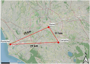
To do this, data from different meteorological stations were used, two airport meteorological stations and one urban station (Figure 1).
The airports stations are reference weather stations for the Meteorological Service of the Military Air Force and for the World Meteorological Organization (WMO) [6].
Figure 1. Locations of the weather stations
The methodological approach of this research can be divided in two main parts:
Starting from this, the first part of the research is characterized by the following steps:
On the other hand, the second part of the research is characterized by the following steps:
The stations selected in this study belong to the Davis Vantage Vue model. In particular, the accuracies of the sensors for measuring wind speed and direction, external temperatures and humidity are respectively 3 km/h or 5%, 3°, 0.5°C and 3%. In terms of resolution, the control unit is characterized by values equal to 1 km/h for wind speed, 1° for wind direction, 0.1°C for external temperature and 1% for relative humidity. Furthermore, Table 1 provides information on their positioning.
Table 1. Acronyms, height above sea level and coordinates of the meteorological stations
|
Stations |
Acronym |
m.a.s.l. |
Coordinates |
|
Fiumicino |
FCO |
3 m |
41°47′53.66″ N, 12°14′22.36″ E |
|
Ciampino |
CIA |
129 m |
41°48′29.49″ N, 12°35′5.82″ E |
|
Rome |
ML15 |
51 m |
42°20′22.402″N,12°24´35.438″ E |
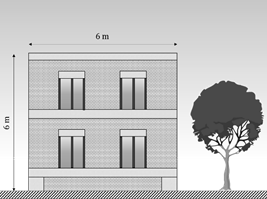
Energy simulations were performed for a simple regular shaped building, characterized by a square plan, with walls with a surface area of 36 m2 (Figure 2). A common wall stratigraphy for the years 1900-1950 was simulated. It is characterized by solid bricks plastered on both sides, with a U-value equal to 1.020 W/m2K. Detailed information about the thicknesses of the layers and the materials’ thermal properties are listed in Table 2.
Table 2. Wall stratigraphy used in simulations
|
Layer |
Thickness [m] |
Thermal conductivity [W/mK] |
Specific heat capacity [J/kgK] |
Mass density [kg/m3] |
|
Plaster |
0.02 |
0.700 |
1000 |
1400 |
|
Solid bricks |
0.58 |
0.770 |
840 |
1600 |
|
Plaster |
0.02 |
0.700 |
1000 |
1400 |
The whole building envelope has a solar absorptance coefficient equal to 0.6. Windows have a total area of 18 m2 and a U-value of 5.61 W/m2K.The infiltration rate was set at 0.5 1/h. Internal heat gains account for occupancy (with sensible heat equal to 65 W and latent heat equal to 55 W) and appliances (thermal power equal to 140 W). The indoor set-point temperatures are 20°C and 26°C for heating and cooling, respectively.
Figure 2. Simplified illustration of the simulated building
3.1 UHI in Rome: Climatic data comparison
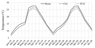
The first step of this study focused on the analysis of temperatures, relative humidity and wind speed values registered by the meteorological stations of Rome, Ciampino and Fiumicino during the years 2019 and 2020 (Figures 3, 4, 5) in order to evaluate the different climatic conditions.
Comparing the average monthly air temperatures, the same trend can be observed from Figure 3 for all three selected stations. In particular, the values obtained from Fiumicino and Ciampino airport stations (renamed in the following figures as “FCO” and “CIA”) are characterized by very similar values during the two years.
On the contrary, air temperatures in Rome are always characterized by higher values, thus confirming the occurrence of the UHI phenomenon within the city.
The Rome meteorological station was appropriately selected not only for the completeness of the data collected, but also for its central position, in a densely built neighborhood of the city center.
Figure 3. Monthly temperature values monitored in Rome, Fiumicino and Ciampino
Fiumicino and Ciampino recorded maximum percentage differences in terms of average monthly temperatures equal to 7% in 2019 and 6% in 2020. Fiumicino was characterized by lower temperatures than Ciampino, especially in the summer months of June, July and August, with temperature differences respectively equal to 1.07°C, 0.74°C and 1°C in 2019, and equal to 0.77°C, 0.94°C and 0.92°C in 2020. In the months of June, July and August, the greatest differences in monthly average temperatures can be noticed analyzing data related to Rome and Fiumicino. Indeed, for these summer months, the monthly differences are respectively equal to 2.68°C, 2°C and 2.29°C in 2019, and 2.05°C, 2.14°C and 1.97°C in 2020. By comparing Rome and Ciampino weather data, the greatest temperature differences can be observed during February 2019 (1.81°C) and February 2020 (1.63°C).
Furthermore, by comparing the average values of the monthly temperatures recorded during 2019 and 2020 by the all stations, very low percentage differences can be observed. In particular, they are equal to 0.1% for the Rome station, 1.1% for the Ciampino station and 0.5% for Fiumicino. This was also confirmed by the analysis of the monthly average temperature differences recorded over the two years for each meteorological station.
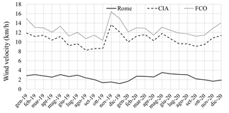
Therefore, the observed temperature trends highlighted the presence of the UHI in Rome. This is also supported by the wind speed analysis (Figure 4). Significant differences occur due to the different positions of the data acquisition points.
Figure 4. Monthly wind velocity values recorded in Rome, Fiumicino and Ciampino
Fiumicino has the highest average wind speed values. During 2019, wind speed values between 10.71 km/h and 16.37 km/h were observed, with an annual mean value of 12.8 km/h. During 2020, values between 11.22 km/h and 14.06 km/h were acquired, with an average wind speed equal to 12.36 km/h. Analyzing Figure 4, wind speeds recorded in Ciampino are higher than those logged in Rome, with an average annual value equal to 10.51 km/h during 2019, and 10.46 km/h during 2020. Instead, Rome is characterized by the lowest wind speed values, with annual averages equal to 2.36 km/h in 2019 and 2.52 km/h in 2020, and maximum peak values of 3.08 km/h in February 2019 and 3.52 km/h in May 2020. The results obtained through the meteorological station located in Rome confirm that the city is characterized by significantly different air circulation flows if compared to neighboring areas as the tall buildings hinder and reduce the wind flows.
The percentage differences relating to the average annual wind speed values recorded by the stations in the two-year period are comparable, with variations equal to 6.6% for Rome, -0.5% for Ciampino and 3.4% for Fiumicino.
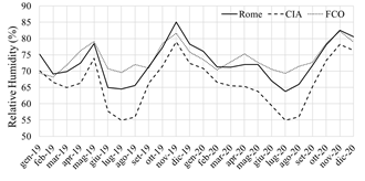
As previously mentioned, the comparisons were also carried out in terms of relative humidity (RH) (Figure 5). Overall, Rome is characterized by lower values than Fiumicino, except for a few months during the winter.
Relative humidity, by reducing the evapotranspiration effect, indirectly contributes to the reduction of urban temperatures. It is known that through evapotranspiration, areas consisting of vegetation, urban agriculture and water bodies can significantly contribute to microclimatic mitigation and therefore to environmental cooling [7].
Figure 5. Monthly Relative Humidity values recorded in Rome, Fiumicino and Ciampino
Fiumicino, due to its position near the Tyrrhenian coast has relatively higher humidity levels during the summer. During 2019, Rome recorded relative humidity values between 64.5% and 85.0%, while in 2020 the percentage range becomes equal to 63.8% and 82.5%, with an annual average of approximately 72.7%. Differently, Fiumicino recorded annual average values of 73.7% in 2019 and 74% in 2020.
Ciampino has the lowest relative humidity, with minimum and average values respectively equal to 54.9% and 66, 6% in 2019 and 54.9% and 66.3% in 2020. In addition, similar trends and particularly comparable annual average values occur in the two years of monitoring, with percentage differences between 0% and 0.5%.
It is worthy to notice that Fiumicino and Ciampino are not actually "rural areas" because they are surrounded by small buildings, albeit with an average height and a different building density.
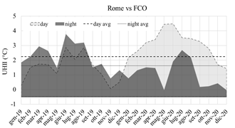
Starting from the temperature data recorded by the climatic control units during the monitoring period, it was possible to determine the monthly Urban Heat Island Index (UHII). This index allows to evaluate the UHI intensity. It was computed during the day and night: for the diurnal UHI intensity, the average maximum temperatures measured in Rome and Fiumicino were used doing the subtraction between the own values; for the nocturnal UHI intensity, the same operation was done using the average minimum measured temperatures (Figure 6). The same procedure was performed comparing Rome and Ciampino (Figure 7).
By comparing 2019 and 2020, the results in terms of UHII show significant differences between the night and day. While in 2019 the greatest differences were reached during the night, in 2020 greater diurnal values were identified.
Analyzing the UHIIs obtained by the comparison between Rome and Fiumicino (Figure 6), in 2019 the maximum nocturnal value was equal to 3.77°C, while the average annual day and night values were equal to 1.45°C and 2.21°C, respectively. In 2020 a different trend can be observed, with maximum differences in diurnal UHII (equal to 4.48°C in June 2020), an average annual daytime value of 3.04°C and a nocturnal value of 1.04°C.
Figure 6. UHII along the two-year monitoring, comparing Rome and Fiumicino stations during the day and night
Furthermore, the percentage differences between the average values of UHII calculated in the two-year registration period are equal to 110% referring to the day and -52.8% referring to the night.
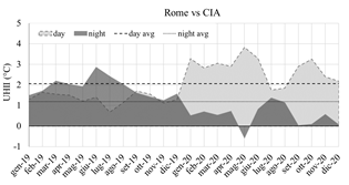
Figure 7. UHII along the two-year monitoring, comparing Rome and Ciampino stations during the day and night
Similar trends, although with different values, was also observed comparing Rome and Ciampino (Figure 7).
In this case the maximum UHII was recorded at night, with a value of 2.87°C (June 2019), while the average annual diurnal and nocturnal values are equal to 1.34°C and 1.87°C, respectively. On the other hand, in 2020 the maximum values of diurnal UHII (equal to 3.83°C) can be observed during May 2020. The average annual diurnal UHII is equal to 2.79°C and the average nocturnal value is 0.50°C. Furthermore, the percentage differences between the average values of UHII calculated in the two-year registration period are equal to 108.4% in the daytime case and -73.4% in the night case.
The evidence of the UHI phenomenon in the city of Rome is due to the presence of neighborhoods characterized by a high building density and tall buildings, which trap radiant heat thus generating urban canyons.
In addition, it is worthy to notice that high pollution levels in the city generate an infrared absorbing layer [8] which prevents thermal radiation from being radiated back from the city. Furthermore, summer air conditioning and therefore the heat generation related to the air-conditioning systems of buildings can further increase urban temperatures [9].
3.2 Influence of different climatic conditions on BES
The second part of the study investigated the influence of various meteorological data on the annual heating and cooling energy needs of a sample building using the dynamic software TRNSYS. For this purpose, the meteorological parameters acquired by the Rome, Fiumicino and Ciampino stations in 2019 were used. The results were then compared with those obtained by applying the Typical Meteorological Years of the IGDG collection, related to Fiumicino and Ciampino (respectively defined as “TMY_ Fiumicino” and “TMY_ Ciampino”) and the climatic data provided by the Italian standard UNI 10349, which was updated in 2016.
By means of a statistical analysis, UNI 10349 provides a typical year composed of data that best represent the typical climatic conditions of a specific location.
The meteorological data acquired by the Rome station in 2019 was used as a reference sample year for the comparison of the results of the energy simulations conducted on the same building model but thermally stressed with the other climatic years. Although the climatic data of both 2019 and 2020 was available, only the climatic data related to 2019 was considered due to the very low differences between the two years. Furthermore, considering as reference 2019 allowed to exclude any effect correlated to the international pandemic of Sars-Cov-2 in terms of heat anthropogenic sources.
Figure 8 shows the comparison between the average monthly temperatures of the sample year and the standard.
Figure 8. Comparison between the sample year and UNI10349 temperature data
It can be observed that the temperature trends of UNI 10349 and the sample year are quite similar from July to December.
The sample year is characterized by slightly higher temperatures except for January, March, and April, during which an inversion of the trend of the two curves can be noticed, with negative temperature differences equal to -0.46°C, -0.65°C and -3.13°C, respectively. Overall, the temperature differences range from -3.13°C to 3.60°C, relating to the months of May and June.
Figure 9 shows a comparison between wind speed and relative humidity values.
The wind speeds reported in UNI 10349 refer to the definition of “wind zone”, considering a subdivision of the Italian peninsula into different zones, characterized by different wind speed values. Rome belongs to “Area C” with an average wind speed of 6.1 km/h and a prevailing South-West wind direction (SW). This value is higher than those obtained in the sample year, whose values range between 1.2 km/h and 3.1 km/h, with an average value equal to 2.4 km/h.
Figure 9. Comparison between the sample year and UNI 10349 wind speed and relative humidity
In Figure 9 it is also possible to observe the trends of the relative humidity values of the Italian standard and the sample year. UNI 10349 shows lower values (from −11% to −40%) compared to the sample year, except for January (+15%), March (+6%) and December (+6%).
Since the weather stations do not measure solar radiation, this data was obtained from the TMYs of the IGDG collection, inside TRNSYS using the “Type 109-TMY2”, specifically considering the TMY of Ciampino and Fiumicino.
In detail, Type 109-TMY2 was used both for the extrapolation of solar radiation values in the energy simulations relating to Rome (Rome 2019), Ciampino (Ciampino 2019) and UNI 10349 and as a complete source of data in the energy model called "TMY_Ciampino".
The same procedure was followed for the simulations related to Fiumicino. The TMY of Fiumicino deriving from the IGDG collection was used both for the acquisition of the missing solar radiation data in the simulation model relating to the year 2019 and as a complete climate file for the simulation of the model "TMY_ Fiumicino".
During the energy simulation through TRNSYS, the wind speed values corresponding to each dataset were also used to compute the external convective heat transfer coefficients, using the well-known correlation $h_{c}=4 \cdot v+4$, where v is the wind speed expressed in m/s [10, 11].
Table 3 summarizes the simulation results in terms of heating and cooling annual energy needs, using the six different climate datasets.
Comparing the data shown in Table 3, significant differences can be noted both in winter and summer.
Table 3. Energy demands of the sample building under different climatic conditions
|
Climatic data |
Heating [kWh/m2] |
Cooling [kWh/m2] |
|
Roma 2019 |
70.4 |
47.7 |
|
Fiumicino 2019 |
88.1 |
25.4 |
|
Ciampino 2019 |
93.8 |
32.1 |
|
UNI 10349 |
91.8 |
31.1 |
|
TMY _Fiumicino |
93.9 |
23.0 |
|
TMY _Ciampino |
104.4 |
24.6 |
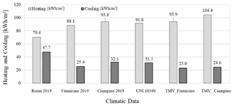
In order to improve the data readability and comparability, the results listed in Table 3 has also been reported as histogram chart in Figure 10.
Figure 10. Heating and cooling annual energy needs under different climatic conditions
Using the climatic conditions observed in Rome during 2019, it is possible to notice the lowest values in terms of energy needs for heating, equal to 70.4 kWh/m2, and the highest for cooling, equal to 47.7 kWh/m2, highlighting that the UHI phenomenon in Rome caused overheating of urban areas compared to peripheral ones, plays a crucial role in assessing the energy demand of buildings.
Table 4 shows the percentage differences obtained for heating and cooling energy needs by comparing the simulation results with the climatic data of the sample year (Rome 2019) to those obtained with the other climatic data.
Table 4. Percentage differences for energy demands using different climatic data
|
Climatic data |
Percentage difference [%] |
|
|
Heating |
Cooling |
|
|
Roma 2019 vs Fiumicino 2019 |
-20.1 |
+87.5 |
|
Roma 2019 vs Ciampino 2019 |
-24.9 |
+48.7 |
|
Roma 2019 vs UNI 10349 |
-23.3 |
+53.3 |
|
Roma 2019 vs TMY _Fiumicino |
-25.0 |
+107.0 |
|
Roma 2019 vs TMY _Ciampino |
-32.5 |
+94.0 |
By comparing the results in terms of heating energy demands, it is possible to observe percentage differences ranging from -20.1% (Fiumicino 2019) to -32.5% (TMY_Ciampino). On the other hand, analyzing the percentage difference related to the cooling energy needs, a much wider range can be observed, from +48.7% (Ciampino 2019) to +107.0% (TMY_Fiumicino).
Starting from this results overview, it is possible to analyze the outcomes listed in Table 4 following two ways.
Considering climatic data related to the year 2019 and taking as reference Fiumicino, it is worthy to observe that climatic conditions outside or inside the city influenced the heating and cooling energy demands with percentage differences equal to -20.1% and +87.5%, respectively. These differences allow to understand the crucial role of meteorological data and their effects on predictions. Modeling a building with airport climate data leads, at best, to percentage differences of -24.9% for heating and +48.7% when they are collected from the Ciampino weather station.
Taking into consideration typical meteorological years such as those provided by the UNI 10349 and the IGDG collection, greater differences can be observed. The comparison among 2019 results and the TMYs allowed to obtain differences ranging between -23.3% and -32.5% for the heating energy demand. This comparison related to the cooling energy need allowed to achieve percentage differences ranging from +53.3% to +107.0%. This comparison highlights the issue of using specific climate data rather than others. The problem is however related to the aim of simulations, if it wants to be predictive or if it must be a simulation of a calibrated model for an energy retrofit.
Similarly, the comparison between the results obtained using the sample year (Rome 2019) and UNI 10349 shows similar percentage variations, with values become equal to -23.3% for heating and 53.3% for cooling.
Finally, analyzing the results listed in Table 4, it is also possible to observe the percentage deviations obtained by comparing the model where the sample year was applied and those performed by the TMYs related to Fiumicino and Ciampino, which are overall higher than the others.
Therefore, the comparison of the achieved simulation results shows very different percentage variations. The resulting deviations are mainly due to the differences in air temperature between the different sites, characterized by different urban textures and green areas, as well as the proximity to the sea. All that can be considered responsible for a significant UHI phenomenon in Rome throughout the year. In conclusion, this analysis revealed the crucial role of climatic data needed to properly reproduce buildings energy performance in terms of heating and cooling energy demands.
This work aimed to quantify the UHI phenomenon of the city of Rome through the analysis, processing and comparison of temperatures, relative humidity and wind speeds collected for two years (2019-2020) by the Ciampino and Fiumicino airport stations and from the weather station located in a central neighborhood of Rome, typical of the urban fabric that characterizes the heart of the city.
The study revealed not negligible differences between the various climatic parameters in the three locations.
Comparing the average monthly air temperatures, the lowest values were observed for Fiumicino, and progressively higher temperatures were registered in Ciampino and, finally, in Rome. The higher temperatures recorded in Rome confirm occurrence of the UHI phenomenon in the city. During summer, the greatest differences in monthly average temperatures were recorded between the stations of Rome and Fiumicino with values equal to 2.68°C in June 2019 and 2.05°C in June 2020. Instead, in the case of the stations of Rome and Ciampino, the greatest temperature differences were recorded in February 2019 (1.81°C) and February 2020 (1.63°C). Also from the analysis of the data relating to wind speed (Figure 3) significant differences emerged based on the different positions in which the stations are located, especially those of Fiumicino and Ciampino airports compared to that of Rome. Fiumicino has the highest average values compared to Ciampino and Rome, registering an average value of 12.6 km/h in the two-year registration period. On the contrary, Rome station recorded the lowest value, with an average of 2.44 km/h. These differences highlighted the influence of the building texture, able to reduce wind flows.
The results revealed significant values of the monthly UHII assumed during the day and night. However, the trends recorded in 2019 differ from those of 2020: while in 2019 the greatest differences were reached during the night, in 2020 there are greater diurnal values. If the climatic conditions are compared to Fiumicino, maximum diurnal and nocturnal UHIIs equal to 4.5°C and 3.8°C can be observed. When this comparison is done taking into consideration Ciampino, the diurnal and nocturnal UHIIs become equal to 3.8°C and 2.9°C, respectively.
Based on the obtained results, in order to countermeasure UHI, it is necessary to consider more suitable cooling strategies in the city. In this regard, the expansion of green areas and the installation of passive building solutions [12] such as green roofs [13, 14] could positively affect urban areas due to their microclimatic action and evaporative cooling. On the other hand, in historical cities (such as Rome), these aspects need to be considered together with architectural constraints.
The effects of the climatic conditions’ variations could have on buildings energy needs were evaluated through TRNSYS. The results in terms of heating energy demands allowed to highlight percentage differences ranging from -20.1% to -24.9% when the reference stations are Fiumicino and Ciampino, respectively. The percentage difference related to the cooling energy needs showed a wider range, from +48.7% to +87.5% when the reference stations are Ciampino and Fiumicino, respectively.
As already mentioned, these results highlight the issue of using specific climate data rather than others. Nevertheless, the problem is related to the aim of simulations. Energy models can be predictive during design phase or they can be used for energy retrofit, but in this case calibrated models are needed.
Therefore, for building energy simulation it is not desirable using meteorological data acquired from airports or peripheral areas (outside the urban fabric) as this could lead to inaccurate estimates of the energy demand of buildings, especially when considering constructions in a high building density neighborhood.
Consequently, there is the need of increasing the number of weather stations within densely built cities, thus providing more localized climatic data, making them available in a simple and immediate manner.
Indeed, such data could be used for the generation of new TMYs based on recent climatic parameters or for multi-year analyses, ensuring better predictive accuracy of building simulation models.
Finally, reliable weather data would also improve the assessments of internal comfort, avoiding the undersizing/oversizing of air-conditioning systems and carrying out more rational assessments of energy retrofit strategies in existing buildings.
From this point of view, future developments will regard a more detailed analysis of the UHI in Rome using much more weather stations and providing assessments also related to the balancing effect due to the reduction in terms of heating energy needs and the growing demands for cooling. It is worthy to investigate how this balancing effect affect users’ costs for heating and cooling, better understanding the existing correlation between economic savings for heating and additional costs for cooling.
The authors would like to thank the meteorological center “METEOLAZIO” for providing the meteorological data used in this study.
[1] Un, I. (2020). Global Status Report for Buildings and Construction (2019). Available at https://www.gbpn.org/china/newsroom/2019-global-status-report-buildings-and-construction.
[2] Ignatius, M., Wong, N.H., Jusuf, S.K. (2016). The significance of using local predicted temperature for cooling load simulation in the tropics. Energy and Buildings, 118: 57-69. https://doi.org/10.1016/j.enbuild.2016.02.043
[3] di Normazione, U.E.I. (2016). UNI 10349-3 Riscaldamento e raffrescamento degli edifici-Parte 3. Differenze di temperature cumulate (gradi giorno) ed altri dati sintetici.
[4] CTI, Comitato Temotecnico Italiano, https://www.cti2000.it/index.php?controller=news&action=show&newsid=34848
[5] TRNSYS Transient System Simulation Tool, (n.d.). http://www.trnsys.com/.
[6] World Meteorological Organization, WMO, (n.d.). https://www.wmo.int/pages/index_en.html.
[7] Qiu, G.Y., Li, H.Y., Zhang, Q.T., Wan, C., Liang, X.J., Li, X.Z. (2013). Effects of evapotranspiration on mitigation of urban temperature by vegetation and urban agriculture. Journal of Integrative Agriculture, 12(8): 1307-1315. https://doi.org/10.1016/S2095-3119(13)60543-2
[8] Lazaridis, M. (2011). First principles of meteorology. In First Principles of Meteorology and Air Pollution, 67-118. https://doi.org/10.1007/978-94-007-0162-5_2
[9] Mayer, H. (1999). Air pollution in cities. Atmospheric Environment, 33(24-25): 4029-4037. https://doi.org/10.1016/S1352-2310(99)00144-2
[10] Evangelisti, L., Guattari, C., Gori, P., Bianchi, F. (2017). Heat transfer study of external convective and radiative coefficients for building applications. Energy and Buildings, 151: 429-438. https://doi.org/10.1016/j.enbuild.2017.07.004
[11] Costanzo, V., Evola, G., Marletta, L., Gagliano, A. (2014). Proper evaluation of the external convective heat transfer for the thermal analysis of cool roofs. Energy and Buildings, 77: 467-477. https://doi.org/10.1016/j.enbuild.2014.03.064
[12] Evangelisti, L., Guattari, C., Grazieschi, G., Roncone, M., Asdrubali, F. (2020). On the energy performance of an innovative green roof in the Mediterranean climate. Energies, 13(19): 5163. https://doi.org/10.3390/en13195163
[13] Asdrubali, F., Evangelisti, L., Guattari, C., Marzi, A., Roncone, M. (2019). Monitoring and dynamic simulation of a pilot building equipped with a green roof. AiCARR Journal, 59(6): 40-44. https://doi.org/10.36164/AiCARRJ.59.06.04
[14] Orsini, F., Marrone, P., Asdrubali, F., Roncone, M., Grazieschi, G. (2020). Aerogel insulation in building energy retrofit. Performance testing and cost analysis on a case study in Rome. Energy Reports, 6: 56-61. https://doi.org/10.1016/j.egyr.2020.10.045