A Calculation Method to Estimate the Thermodynamic Performance of Solar Tower Power Plants with an Open Air Brayton Cycle and a Combined Cycle

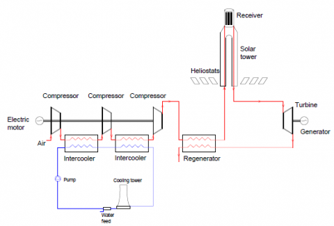
Figure 1 schematically shows the concentrating solar tower power plant with an open air Brayton cycle. It consists of an inter-refrigerated multistage compressor and a regenerator. The air drawn from the atmosphere is compressed by a three inter-cooled stadiums compressor, preheated in the regenerator and sent into the receiver placed on top of the solar tower, from which it exits at high temperature. Afterwards, it is sent to the gas turbine connected to the electric generator, and before being discharged to the atmosphere, the air passes through the regenerator. A cooling tower is used to refrigerate the water used in the cooling circuit.

1.png

Figure 1. Scheme of a solar tower power plant with an open air Brayton cycle

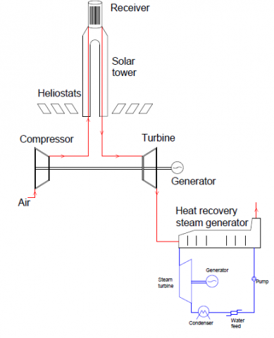
Figure 2 refers to the combined cycle. It consists of a topping Brayton cycle, a heat recovery boiler and a bottoming Rankine cycle. The compressor sends the air directly into the receiver. The air at high temperatures drives the gas turbine. Afterwards, it is sent to a heat recovery steam generator, where superheated steam is produced and used to drive the steam turbine.

2.png

Figure 2. Scheme of the Brayton-Rankine combined cycle plant

In both systems, a constant turbine inlet temperature (TIT) equal to 1000°C is considered, while the flow rate varies depending on the direct normal radiation (DNI). In any case, the air flow rate should not be lower than 60% of its nominal design value, in order to not degrade excessively the isentropic efficiency of the compressor. When the flow rate reaches its minimum value, it is kept constant as the DNI decreases. This determines a reduction of the turbine inlet temperature, up to a minimum value to 600°C, for which the plant can still produce electricity.

The operation of the components of the two systems was simulated by the THERMOFLEX code [30], starting from the design conditions, see table 1 and table 5 and then evaluating their performances in off-design conditions, by varying the inlet temperature of the air and the opening of the Inlet Guide Vanes (IGV) of the compressor, so as to vary the air flow rate.

Based on the results obtained, some correlations have been developed for the key variables, such as the air temperature at the compressor exit in the combined cycle plant (or at the regenerator exit in the Brayton cycle) and the thermodynamic efficiency of the gas and steam turbines in the combined cycle (or of the gas turbine in the Brayton cycle).

At low solar irradiance, the plants are operated at constant flow rate, the correlations developed concerned the thermal power transferred to the fluid in the receiver, the air temperature at the inlet of the turbine, and the thermodynamic efficiency of the turbines.

All these correlations, along with a simulation model of the heliostat field and the tower receiver, were implemented in a Matlab calculation algorithm, called TERSOLTO (thermodynamic solar tower) in the B and CC versions, respectively valid for the Brayton cycle and the combined cycle.

Through TERSOLTO, starting from the values of direct solar irradiance, air temperature and humidity, the hourly values of the electrical power generated by the plants, the average hourly and annual values of the efficiency and the electricity produced in a year can be calculated.

In the following paragraphs the models and correlations used are described in detail.

2.1 Calculation model of the Brayton Cycle

Table 1 reports the plant design data. The main input data are: the rated electrical power, the atmospheric air temperature, the DNI design value, the inlet temperature to the gas turbine, the pressure ratio of the compressor and the turbine.

Once defined the type of system and characteristics of the various components, the THERMOFLEX code considers the receiver as a generic heat generator, and allows to calculate the nominal air flow rate. Hence, it is possible to obtain the desired net electrical power, the thermal power supplied from the receiver to the fluid, the gross and net electrical power supplied from the gas turbine, the net thermodynamic efficiency of the cycle and many other variables of interest.

By means of the THERMOFLEX code, after determining the above mentioned variables in design conditions, calculations in off-design conditions were performed, considering: three different values of the atmospheric air temperature of 0°C, 25°C and 50°C; three opening values of the IGV, of 100%, 80% and 60%; and maintaining the turbine inlet temperature constant at 1000°C.

Table 2 reports the values of air flow rate, air temperature at the regenerator exit, the heat transferred from the receiver to the fluid, the net efficiency of the power block and the net electrical power plant production, for different outside air temperatures and IGV.

Table 1. Design data of Air Brayton Solar Tower Power Plant located in Almeria

The correlations obtained are the following:

for T_A=0℃,

$T_{o r}=a+b \cdot x^{3}+c / x$            (1)

with a=459.561; b=-12.78871; c=43.25952

$\eta_{g t}=a+b \cdot x+c x^{0.5}$        (2)

with a=-0.49634; b=-0.85800; c=1.7696

for T_A=25℃,

$T_{o r}=a+b \cdot x^{3}+c / x^{1.5}$        (3)

with a=486.42211; b=-17.80170; c=22.19127

$\eta_{g t}=a+b \cdot x+c x^{0.5}$         (4)

with a=-0.550466; b=-0.895711; c=1.85013

for T_A=50℃,

 $T_{o r}=a+b \cdot x^{3}+c / x$       (5)

with a=462.57941; b=-13.297368; c=43.1433

$\eta_{g t}=a+b \cdot x+c \cdot x^{0.5}$        (6)

with a=-0.61494; b=-0.94732; c =1.94717

The proposed correlations present a correlation index of 99.99% and a maximum error of less than 0.5%.

They have been implemented in the TERSOLTO-B algorithm, in which meteorological data of the sites where the plants are located (outside air temperature, relative humidity, DNI, etc.) are available. At any time, the flow rate value (m), which ensures an outlet temperature of the receiver of 1000°C, can be obtained, using the heat balance equation between the solar thermal power supplied by the field of heliostats and the heat received by the fluid in the receiver, with an iterative method.

The balance equation is:

$\mathrm{SM} \mathrm{A}_{e} \mathrm{DNI} \eta_{o p t}-P_{l o s s}=\mathrm{m}\left(\mathrm{H}\left(\mathrm{T}_{o R}\right)-\mathrm{H}\left(T_{o r}\right)\right)$      (7)

where SM is the solar multiple, A_e is the total area of the heliostats, $\eta_{\text {opt}}$ [32] is the optical efficiency of the heliostats field, taking into account the reflection coefficient of the mirrors, the transmissivity of the atmosphere, the cosine, shadowing, blocking, and spillage effects of the individual heliostats and the absorption coefficient of the receiver, P_loss is the sum of the radiative and the convection losses of the receiver, m is the fluid flow rate, H(T_OR) is the enthalpy of the fluid at the outlet of the receiver and H(T_or) is the enthalpy of the fluid at the outlet of the regenerator.

The radiative loss P_loss was evaluated by the equation:

$P_{\text {rad}}=A_{R} \varepsilon_{R} \sigma\left(T_{R}^{4}-T_{A}^{4}\right)$        (8)

where, A_R is the area of the receiver, $\sigma$ is the emissivity of the receiver, σ is the Stephan-Boltzmann constant, T_R is the temperature of the receiver and T_A is the temperature of atmospheric air. For simplicity, it is assumed that the temperature of the receiver is uniform and equal to the turbine inlet temperature.

The convective loss is instead calculated using the equation:

$P_{\text {conv }}=h A_{R}\left(T_{R}-T_{A}\right)$        (9)

where, h is the convective heat transfer coefficient between the receiver and the outside air. Normally, for high temperatures of the receiver, the convective loss is negligible compared to the radiative one.

Starting from the initial value of x=1 (valid in design conditions), at the considered hour, for the outside air temperature value an initial value of the outlet temperature from the regenerator is calculated by interpolation, using Eqns. (1), (3) and (5). Considering the quality of moist air, the enthalpies H(T_OR) and H(T_or) are calculated and, by Eq. (7), an initial value for the air flow rate and the parameter x are obtained. This procedure is repeated until x reaches convergence and for the final value of x the gas turbine efficiency and the electrical power delivered by the plant are calculated.

When the thermal power transmitted from the receiver to the Power Block is larger than 136 MW, 10% higher than the nominal design value, part of heliostats is supposed to defocus, so as not to exceed this maximum power value. Hence, the maximum value of the dimensionless parameter x is 1.1.

When the x value is lower than 0.6 (60% of the nominal flow rate), for low values of DNI, it is assumed, as already stated, that the flow rate is kept constant, and the plant operates with a variable TIT up to a minimum value of 600°C.

To determine the TIT under these conditions, a further series of calculations were carried out by THERMOFLEX code, maintaining the fluid flow rate constant and varying the TIT between 1000°C and 600°C. From the data obtained, the following correlations for the TIT (Q) and the gas turbine efficiency $\eta_{g t}$ (TIT) were developed:

for T_A=0℃,

$T I T=a+b \cdot Q^{0.5}+c / Q$           (10)

with a=317.763; b=82.5716; c=203.540

 $\eta_{g t}=a+b \cdot T I T^{0.5}+c / T I T^{2}$         (11)

with a=0.63151; b=-2.70358•10^-3; c=-187992.161;

for T_A=25℃,

$T I T=a+b \cdot Q^{0.5}+c / Q$            (12)

with a=318.95934; b=82.03883; c=198.48652

 $\eta_{g t}=a \cdot T I T^{3}+b \cdot T I T^{2}+c \cdot T I T+d$        (13)

with a=3.7425•10^-9; b=-1.0478•10^-5; c=1.0245•10^-2; d=-3.1633

for T_A=50℃,

$T I T=a+b \cdot Q^{0.5}+c / Q$          (14)

with $a=317.92342 ; b=82.0407 ; c=209.2899 ;$

$\eta_{g t}=a+b \cdot T I T^{0.5}+c / T I T^{2}$         (15)

with a=0.458811; b=3.118367•10^-11; c=209.2899

In the above equations Q is the thermal power transferred to the fluid in the receiver.

All correlations present a correlation index of 99.99% and a maximum error of less than 0.5%.

The calculation of the total area of the heliostats A_e, of the height of the tower, of the size of the receiver, of the average optical efficiency of the heliostats $\eta_{o p t}$, see Eq. (7), has been carried out by the DELSOL-3 code [33], assuming a configuration of the Surround-field type and an outer cylindrical receiver, using an optimization procedure of the field-receiver system performance. For the value of SM=1, in the design conditions, summarized in Table 1, the following values were obtained: an area of the heliostats field of 302,499 m², a tower height of 102.5 m, a 6.615 m receiver diameter and a receiver height of 8.818 m.

The values of the optical efficiency, calculated by DELSOL-3 code for SM 1.2, as a function of the zenith and azimuth angle of the sun, are given in Table 3.

The optical performance of heliostats can be evaluated at any time of the day and month for interpolation. This calculation is made by the TERSOLTO program.

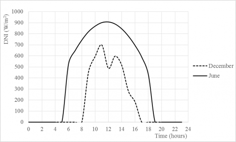
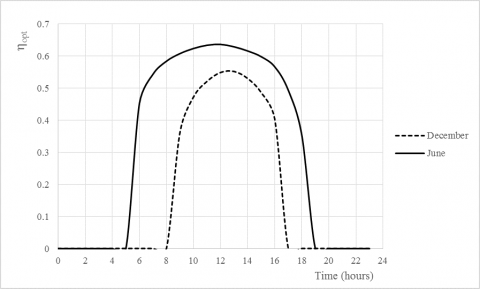
Figures 3-5 show, for the same value of the solar multiple, for a clear day in June and an intermediate day in December, the time trends of DNI, of optical efficiency of the heliostats field and of net electrical power.

Table 3. Optical efficiency of the solar field of the Brayton Cycle Plant for SM=1.2 as a function of sun zenith and azimuth angles

3.png

4.png

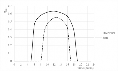
Figure 4. Heliostat optical efficiency as a function of the time in the Brayton Cycle

5.png

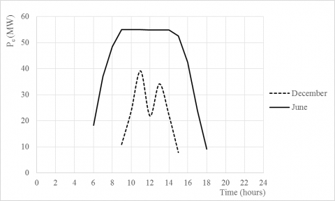
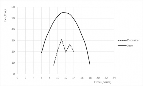
Figure 5. Electrical Power as a function of time in the Brayton Cycle plant

Table 4. Annual data of Brayton Cycle Plant

2.2 Calculation model of the combined cycle

Table 5 reports the design data of the solar tower power plant with a combined cycle.

Table 5. Design data of the Solar Tower Power Plant with Combined Cycle located in Almeria

Table 6. Influence of IGV aperture and of inlet air temperature on the performance of the CC plant

for T_A=0℃,

$T_{o c}=a+b \cdot x^{3}$          (16)

with a=246.5919; b=90.25454;

$\eta_{g t}=a+b / x^{2}$       (17)

with a=0.308604; b=-3.373074•10^-2

$\eta_{s t}=a+b / x$       (18)

with a=0.103356; b=-6.824015•10^-2

for T_A=25℃,

$T_{o c}=a \cdot b^{x}$       (19)

with a=204.3563; b=1.85103;

$\eta_{g t}=a+b / x^{2}$       (20)

with a=0.300301; b=-3.125406•10^-2;

$\eta_{s t}=a \cdot x^{b}$       (21)

with a=0.182133; b=-0.414489;

for T_A=50℃,

$T_{o c}=a \cdot b^{x}$     (22)

with a=255.1888; b=1.60495

$\eta_{g t}=a+b / x$          (23)

with a=0.38281; b=-0.112634

$\eta_{s t}=a \cdot b^{x}$       (24)

with a=0.347898; b=-0.545025

For a constant flow rate operation and variable TIT the following correlations were obtained:

for T_A=0℃,

$T I T=a \cdot Q^{3}+\cdot Q^{2}+c \cdot Q+d$       (25)

with a=5.898722•10^-5; b=-2.019249•10^-2; c=10.918839; d=190.248464

$\eta_{g t}=a+b \cdot T I T^{0.5}+c / T I T^{1.5}$       (26)

with a=0.326549; b=-1.445094•10^-7; c=-3228.2688;

$\eta_{s t}=a \cdot T I T^{3}+b \cdot T I T^{2}+c \cdot T I T+d$             (27)

with a=8.33333•10^-11; b=-6.214285•10^-7; c=10.918839•10^-3; d=-0.296885

for T_A=25℃,

$T I T=a \cdot Q^{3}+b \cdot Q^{2}+c \cdot Q+d$        (28)

with a=7.86633•10-5; b=-2.38838•10-2; c=11.733322; d=214.908106

$\eta_{g t}=a+b \cdot T I T+c / T I T^{1.5}$           (29)

with a=0.323386; b=-7.309416•10^-6; c=-3214.9926

$\eta_{s t}=a+b \cdot T I T^{2}+c \cdot T I T^{0.5}$           (30)

with a=-0.480034; b=-1.443485•10^-7; c=2.629234•10^-2

for T_A=50℃,

$T I T=a+b \cdot x^{0.5}+c / x^{0.5}$       (31) 

with a=-1013.990342; b=205.346943; c=2663.537571

$\eta_{g t}=a+b \cdot T I T^{0.5}+c / T I T^{2}$       (32)

with a=0.147127; b=3.3784093•10^-3; c=-66915.18

$\eta_{s t}=a \cdot T I T^{2}+b \cdot T I T+c$          (33)

with a=-0.0000003; b=-6.99999•10^-4; c=-0.149

All above correlations present a correlation index of 99.99% and a maximum error less than 0.5%.

The maximum thermal power transmitted from the receiver to the power block, in this plant, is 122 MW.

Using DELSOL-3 code, the total area of the heliostats A_e, for SM = 1, in the design conditions of Table 5, resulted to be 273,784 m²; the height of the tower and the size of the receiver resulted equal to those of the Brayton cycle plant.

The values of the optical efficiency, calculated by DELSOL-3 code for SM = 1.2, as a function of the zenith and azimuth angle of the sun, are given in Table 7.

Figures 6-7 show the optical efficiency of the heliostats field and the net electrical power as functions of time for the same value of the solar multiple, for a clear day in June and an intermediate day in December.

6.png

Figure 6. Heliostat optical efficiency as a function of time in the Combined Cycle plant

7.png

Figure 7. Electrical power as a function of time in the Combined Cycle plant

Table 8. Annual data of CC Plant

Tables 1 and 2, containing the design data of the two systems, show that a 50 MW electrical power plant can be obtained, in the case of the combined cycle, with a heliostats area of 273,784 m², against an area of 302,499 m² in the case of the Brayton cycle, with a reduction of 11%.

This is mainly due to the difference between the thermodynamic net efficiency of the power block, which is 0.449 in the combined cycle and 0.404 in the Brayton cycle.

The annual electricity supplied by the combined cycle is 109,538 MWh, against a value of 97,943 MWh in the Brayton cycle, with an increase of about 12%. The capacity factor is 25% in the combined cycle, compared with 22.4% of the Brayton cycle. The average annual plant efficiency is 16.3% in the combined cycle against the 13.2% of the Brayton cycle.

The 50 MW plant using molten salts, with an area of heliostats of 247,497 m² (lower than both the Brayton plant and the combined Brayton cycle for the smaller radiative losses from the receiver), provides an annual electrical energy, see table 9, of 61,022 MWh for SM = 1.

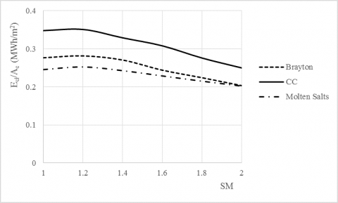
Figure 8 shows the annual energy per square meter obtained with the three systems, as a function of the solar multiple: the graph shows that the maximum value is obtained for SM = 1.2 and is 0.282 MWH/m² for the Brayton plant, 0.351 $\mathrm{MWh} / \mathrm{m}^{2}$ for the combined cycle plant and 0.253 MWH/m² for the plant using molten salts. Therefore, the specific energy of the Brayton plant is 11.5% greater than that obtained for the plant using molten salts, while for the combined cycle there is an increase of 38.7% with respect to the system using molten salts.

8.png

Figure 8. Annual Electrical Energy per square meter of heliostat as a function of solar multiple

Based on these results, it is evident that the technical performance of the combined cycle is superior to that of the Brayton cycle, and both of these systems have better performances than the plant using molten salts.