OPEN ACCESS
Solar chimney is a technology used to regulate the heat flow between indoor and outdoor of a building. It employs solar radiation to increase the temperature of the air for optimize its circulation and by improving its quality. In this paper, a numerical investigation on a prototypal solar chimney system integrated in a south facade of a building is presented. The chimney is 4.0 m high, 1.5 m wide whereas the thickness at the inlet the channel has a gap equal to 0.34 m and at the outlet it is 0.20 m. The chimney consists of a converging channel with one vertical wall and one inclined of 2°. The analysis is carried out on a three-dimensional model in airflow and the governing equations are given in terms of k-ε turbulence model. The problem is solved by means of the commercial code Ansys-Fluent. The simulations are carried out considering the solar irradiance for assigned geographical location and for a daily distribution in four different days, one for each climatic season. Further, comparison between the different results obtained by operating in quasi – steady state regimes is examined and discussed. Results are given in terms of wall temperature distributions, air velocity and temperature fields and transversal profiles in order to evaluate the differences between the different configurations and thermal and fluid dynamic behaviors.
integrating solar system, chimney effect, natural ventilation, building envelope
The Solar chimney is a zero environmental impact system studied and designed to improve the natural ventilation of the dwellings, exploiting the convention of heated air with passive solar energy. Invented by the ancient Persians, this extraordinary intuition was also used by the ancient Romans who optimized its potentialities, not only to ventilate the rooms, but also to capture the light and spread it in all the environments.
A solar chimney is a type of passive solar heating and cooling system that can be used to regulate the temperature of a building as well as providing ventilation. Essentially, solar chimneys are hollow containers that connect the inside part of the building to the outside part of the building.
Solar chimneys are easy and inexpensive means to heat and ventilate a building. First, a chimney is built and coated in some dark or black material. It is colored black because this minimizes the amount of sunlight that is reflected from the chimney, absorbing more of the heat and ensuring more of the heat is transferred to the air inside the building.
As well, these chimneys are generally placed on a South facing wall if the home is in the Northern hemisphere. For this reason, in the construction of a solar chimney do not matter its size or the diameter of its ducts, but the portion of surface that receives the solar radiation.
The process of heating a space using a solar chimney is fairly simple. When the solar radiation hits the side of the chimney, the column of air inside the chimney is heated. If the top exterior vents of the chimney are closed, the heated air is forced back into the living space. This provides a type of convective air heating. As the air cools in the room it is pulled back into the solar chimney, heating once again.
Cooling a space using a solar chimney is made possible by two vents. The first vent is at the top of the chimney. The second is at the opposite end of the building, providing an opening between the building and outside air to allow for ventilation. When solar radiation hits the side of the chimney, the column of air inside the chimney is again heated. The vent at the top of the chimney is kept open so this heated air is not trapped. This heated air is pulled up and out of the chimney, pulling new air in from the outside and creating a sort of flow that provides cool, renewed air into the building.
Therefore, the advantages of installing a solar chimney are numerous and valid at any time of the year: the costs related to air conditioning are cut down, opting for an innovative and low energy impact solution. Also, the system doesn’t use fossil fuels but clean energy that improves air ventilation in the house especially in smaller environments, or in those that do not have openings or windows.
Since the first proposal of solar chimney in 1980, several studies were carried out in order to know and optimize the main features of this technology [1-2]. Such as: Vieira et al. [3] carried out a numerical analysis to investigate the influence of geometry and different soil temperatures on the power of the plant. Shirvan et al. [4] studied a two-dimensional axial symmetric model of a solar chimney in Zanjan (Iran), identifying collector and chimney geometry values for maximum power. Hua et al. [5] numerically compared energy production capacities of a divergent solar chimney, a cylindrical chimney with divergent outlet and cylindrical chimney with divergent inlet. In [6], Hua et al. analyzed effects of geometry of a divergent solar chimney on power and aerodynamic. In [7], Hua et al. analyzed the performance of a diverging solar chimney by considering two geometric parameters: the ratio of inlet and outlet areas of chimney and wall inclination. Ayadi et al. [8] studied performance of a solar chimney by varying the inclination of the collector roof. Ayadi et al. [9] analyzed geometric factors optimizing chimney performance. Gholamalizade and Kim [10] numerically analyzed the model of Manzanares solar chimney equipped with an inclined wall. Esfidani et al. [11] studied a geometric optimization method for solar chimney system. Bahar et al. [12] simulated a solar chimney in different areas of Tunisia. Sudprasert et al. [13] analyzed the effects due to humidity on solar chimney performances. Bianco et al. [14] carried out an experimental and numerical survey on natural air convection through a converging vertical channel, uniformly heated, to analyze radiative effects on heat exchange, considering two investigated emissivity values. Langellotto and Manca [15] studied the phenomenon of natural convection within a converging, uniformly heated vertical channel. Manca et al. [16-17] numerically surveyed natural convection inside a divergent, vertical, uniformly heated channel, under laminar regime. Buonomo et al. [18-19] carried out a numerical survey on natural air convection in a convergent vertical channel. Cirillo et al. [20] carried out a numerical and experimental analysis on a solar chimney integrated on the south wall of a building. Zha et al. [21] studied the performance of a solar chimney in a building located in the eastern part of China (Shanghai). Coppi et al. [22] conducted a numerical survey on performance of a solar chimney integrated in the center of a building in Rome, in which a horizontal plate at the base of the building works as a thermal reservoir. Montelpare et al. [23], knowing power plant of Manzanares, calibrated a numerical model based on finite volumes to design a solar tower with reduced dimensions and they conducted an analysis on various geometric parameters. Bouabidi et al. [24] investigated the effect of the chimney configuration on the solar chimney power plant performance. The influence of the inlet shape of the solar air collector on the solar chimney performance was investigated experimentally and numerically by Al-Kayiem et al. [25]. Hassan et al. [26] performed a parametric 3-D CFD analysis of solar chimney power plant. Ahmed and Hussein [27] realized two similar experimental models of solar chimney including both PV panels with solar chimney plant for electricity generation. Buonomo et al. [28] investigated on a prototypal solar chimney system integrated in a south facade of a building.
In this work a numerical investigation on a prototype solar chimney system integrated in a south facade of a building is presented. The chimney is formed by a converging channel with one vertical wall and one inclined wall. The numerical analysis is carried out on a three-dimensional model and the governing equations are given in terms of k-ε turbulence model. The analyses are made in four different days of the year and the results are provided in terms of wall and glass temperature distributions, air velocity and mass flow at the outlet.
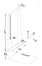
In Figure 1 is reported the investigated configuration. It consists of a channel composed by a vertical wall of height L, on which is imposed a uniform heat flux, and by a glass wall, inclined to the vertical at an angle α. Inlet and outlet sections are bmax and bmin respectively, and depth is equal to W. The distance of inlet chimney section from the ground is H. In Table 1 are reported the geometric values.
Figure 1. Solar chimney scheme
Table 1. Solar chimney dimensions
|
Dimension |
Value |
|
L |
4.00 m |
|
H |
1.00 m |
|
bmax |
0.34 m |
|
bmin |
0.20 m |
|
W |
1.50 m |
In solar chimney the natural convection flow is considered steady, turbulent and three-dimensional. Density in buoyancy force is modeled by Boussinesq formulation and all thermo-physical fluid properties are assumed invariant with temperature and they are evaluated at ambient temperature, T0, equal to 300 K in all cases. Ambient is assumed as a black body at temperature of 300 K. Compression work and viscous dissipation are assumed negligibly small. Therefore, the governing equations can be written as:
Conservation of mass:
$\bar{∇}∙\bar{V}=0$ (1)
Conservation of momentum:
$\rho \bar{V}\cdot \bar{\nabla }\bar{V}=\rho \bar{g}-\bar{\nabla }p+\bar{\nabla }\bar{\bar{\tau }}$ (2)
with τ the viscous stress tensor.
Conservation of energy:
$ρc_p\bar{V}∙\bar{∇}T=λ∇^2T$ (3)
In the present work is considered k-ε model proposed by Launder and Spalding [29]. This model is correlated to the natural convection in high chimney, as suggest by Ayadi et al [8-9]. Turbulent dynamic viscosity is calculated from the knowledge of kinetic energy of turbulence, k, and turbulent kinetic energy dissipation rate, ε, given from the following equations:
$μ_t=ρ∙C_μ∙f_μ∙(\frac{k^2}{ε})$ (4)
Turbulence kinetic energy (k-equation)
$\frac{∂}{∂x}(ρ\bar{u}k)+\frac{∂}{∂y}(ρ\bar{v}k)+\frac{∂}{∂z}(ρ\bar{w}k)=\frac{∂}{∂x} [(μ+\frac{μ_t}{σ_k}) \frac{∂k}{∂x}]+\frac{∂}{∂y}[(μ+\frac{μ_t}{σ_k}) \frac{∂k}{∂y}]+\frac{∂}{∂z} [(μ+\frac{μ_t}{σ_k} \frac{∂k}{∂z}]+ G_k+ G_b- ρε–D$ (5)
Turbulence dissipation (ε-equation)
$\frac{∂}{∂x} (ρ\bar{u}ε)+\frac{∂}{∂y} (ρ\bar{v}ε)+\frac{∂}{∂z} (ρ\bar{w}ε)=\frac{∂}{∂x} [(μ+\frac{μ_t}{σ_ε}) \frac{∂ε}{∂x}]+\frac{∂}{∂y} [(μ+\frac{μ_t}{σ_ε}) \frac{∂ε}{∂y}]+\frac{∂}{∂z} [(μ+\frac{μ_t}{σ_ε}) \frac{∂ε}{∂z}]+C_s1 f_1 \frac{ε}{k} (G_k+G_s3 G_b )-C_s2 f_2 \frac{ε^2}{k}+E$ (6)
In equations (5) and (6), the first two terms represent, respectively, transport of kinetic energy of turbulence and dissipation rate of kinetic energy by convection. Third and fourth terms represent transport of these quantities by diffusion. Gk represents the rate of generation of turbulent kinetic energy due to mean velocity gradients. ρε is the destruction rate of turbulent kinetic energy and Gb is the rate of generation of turbulent kinetic due to buoyancy. In addition, there are some extra terms denoted by D in k-equation and E in ε-equation to explain the behavior near the wall.
The external reservoir (at the inlet section) is the zone of the computational domain considered in order to simulate the diffusion of momentum and energy that occur outside the channel. Ambient pressure and temperature are assumed at inlet and outlet sections. Is considered the acceleration of gravity and its value is set equal to 9.81 m/s2. A uniform heat flux on the heated surface is considered, while the unheated surfaces are considered adiabatic. For unsteady energy and momentum equations it is chosen the second-order upwind scheme. The Semi- Implicit Method for Pressure-Linked Equations (SIMPLE) scheme is chosen to couple pressure and velocity, in addition the diffuse transfer radiation model (DTRM) is considered, assuming all surfaces to be diffuse [30-31]. This involves that the reflection of incident radiation at the surface is isotropic with respect to the solid angle. Therefore, scattering effect is not taken into account. The equation for the exchange of radiation intensity of DTRM, dI, along path ds can be written as:
$\frac{dI}{ds}+αI=\frac{ασT^4}{π}$ (7)
where: α is gas absorption coefficient; I is the total radiation intensity and it depends on position (r) and direction (s); T is gas local temperature; σ is the Stefan-Boltzmann constant and it is equal to 5.672·10-8 W/ (m2·K4). Refractive index is assumed unitary. The DTRM integrates the equation (6) along a set of rays that leave outer walls. Mainly, the number of rays traced and the computational grid limit model’s accuracy. However, the number of divisions of the solid angle is obtained thanks to appropriate analysis, as required by the chosen radiation model (DTRM). The goal is to achieve a compromise between reliability of results and containment of calculation time.
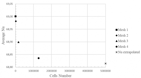
Thanks to the software Gambit [32], geometric model and mesh of the computational domain are realized. In particular, creating the mesh, several grids were realized and compared, depending on Richardson's extrapolation equation. Consequently, the chosen of a grid that counts 160000 calculation cells [33], which represents the optimal compromise between the accuracy of the simulation and the duration of the calculation time. Table 2 reports the number of calculation cells N and the values of Nusselt Number. Figure 2 shows the percentage error.
Table 2. Percentage error of Nusselt number
|
Mesh |
Cells |
Nu |
Err % |
|
1 |
2500 |
69.00 |
0.27% |
|
2 |
20000 |
68.98 |
0.24% |
|
3 |
160000 |
68.90 |
0.12% |
|
4 |
1280000 |
68.84 |
0.03% |
|
Asymptotic value |
|
68.81 |
|
Figure 2. Percentage Nusselt number error
The investigated configuration consists of a channel composed by a vertical aluminum wall, on which is imposed a uniform heat flux, and by an inclined glass wall. Heated wall is oriented towards south and simulations are performed considering the solar chimney located in Aversa (Italy) during the solstices (June 21 in summer, December 22 in winter) and the equinoxes (March 20 in spring, September 23 in autumn). The next table reports the sunrise-sunset calendar for each considered day:
Table 3. Sunrise-sunset calendar during the solstices and the equinoxes
|
Day |
March 20 |
June 21 |
September 23 |
December 22 |
|
Sunrise [h] |
6:10 |
5:30 |
6:50 |
7:30 |
|
Sunset [h] |
18:10 |
20:38 |
19:00 |
16:30 |
In every day that was analyzed, the solar chimney has the same configuration: it is composed by a vertical wall and an inclined wall. Different values of heat flux are applied, considering different hours of each days, from sunrise to sunset, in quasi-steady state regime.
Inclined wall is a low-emissivity glass (ε=0.84, 0.04 external and internal surface, respectively). This sort of glass has a coating to oppose heat loss: solar heating can enter in the structure and energy produced by inner radiating surfaces cannot exit.
Next table reports values of heat flux due to radiation from sunrise to sunset of every hour. It is possible to note that when the Sun is on the peak of his path, the values of Direct Normal Solar Irradiation are higher respect to the dawn position and dusk position. Particularly, the upper values are between the 12:00 and 13:00.
Table 4. Direct Normal Solar Irradiation (D.N.S.I.) due to solar radiation, W/m2
|
21-June |
22-December |
23-September |
20-March |
||||
|
Hour |
D.N.S.I |
Hour |
D.N.S.I |
Hour |
D.N.S.I |
Hour |
D.N.S.I |
|
5:30 |
296.113 |
|
|
|
|
|
|
|
6:30 |
592.512 |
|
|
6:50 |
429.313 |
6:10 |
0 |
|
7:30 |
729.364 |
7:30 |
0 |
7:50 |
708.617 |
7:10 |
530.787 |
|
8:30 |
801.544 |
8:30 |
481.649 |
8:50 |
822.451 |
8:10 |
784.031 |
|
9:30 |
842.424 |
9:30 |
732.958 |
9:50 |
877.668 |
9:10 |
885.950 |
|
10:30 |
865.285 |
10:30 |
831.127 |
10:50 |
904.497 |
10:10 |
935.161 |
|
11:30 |
875.937 |
11:30 |
868.935 |
11:50 |
913.374 |
11:10 |
958.748 |
|
12:30 |
876.716 |
12:30 |
869.943 |
12:50 |
907.214 |
12:10 |
965.952 |
|
13:30 |
867.783 |
13:30 |
834.696 |
13:50 |
884.006 |
13:10 |
959.161 |
|
14:30 |
847.210 |
14:30 |
741.587 |
14:50 |
8.5.087 |
14:10 |
936.128 |
|
15:30 |
809.927 |
15:30 |
505.343 |
15:50 |
735.531 |
15:10 |
887.932 |
|
16:30 |
744.381 |
16:30 |
0 |
16:50 |
501.014 |
16:10 |
788.44 |
|
17:30 |
622.191 |
|
|
17:50 |
0 |
17:10 |
543.556 |
|
18:30 |
363.170 |
|
|
18:50 |
0 |
18:10 |
0 |
|
19:30 |
0 |
|
|
|
|
|
|
|
20:30 |
0 |
|
|
|
|
|
|
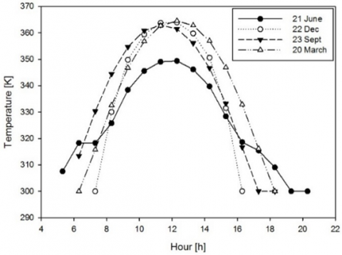
In the next Figures 3-6, the trend of some thermo-fluido-dynamic characteristics is shown for each hour of the day. Twall,max and Tglass max are the maximum temperature of the vertical wall and the inclined glass, respectively; vmax is the maximum value of velocity in the channel and ṁ is the mass flow rate in the channel. Values grow in the morning and they are higher at 12:00; then values decrease, because solar radiation is lower. Trends are various in the different positions of Sun. In all analyzed day, the shape of the trend is similar; there is a maximum value between the 12:00 and 13:00 for each day. Indeed, the maximum values on the wall are equals about to:
Figure 3. Maximum temperature trend of the wall during the equinoxes and solstices
350 K on 21 June, 364 K on 22 December, 363 K on 23 September, 365 K on 20 March. For the glass, at same time, the maximum values are equals to 315 K on 21 June, 315 K on 22 December, 317 K on 23 September, 317 K on 20 March. In each simulation, temperature values grow along the wall, but they are lower on the bottom of it, because solar rays reach this part more difficultly. As shown, especially from 10:00 to 14:00, vmax and ṁ have similar values during the day. At the 18:00 for 21 June, at the 15:00 for 22 December and at the 17:00 for 29 September and 20 March, it is possible to detect.
Figure 4. Temperature trend of the glass during the equinoxes and solstices
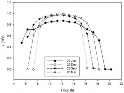
Figure 5. Maximum velocity values at outlet section during the equinoxes and solstices
Table 5. Percentual decreases of vmax and ṁ
|
|
June 21 |
December 22 |
September 29 |
March 20 |
|
Δv [%] |
40 |
22 |
35 |
36 |
|
Δṁ [%] |
45 |
26 |
41 |
43 |
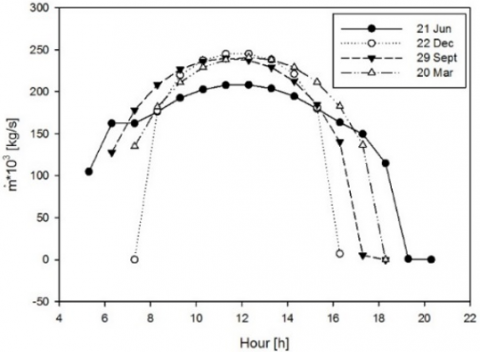
Figure 6. Mass flow rate values at outlet section during the equinoxes and solstices
Largest differences and by comparing with values at the 12:00, it is possible to note these values decrease. For the percentual decreases of vmax and ṁ, it was considered, for both values, this formula:
$∆%=(\frac{value at sunset-value at the 12:00}{value at the 12:00})∙100$ (8)
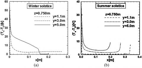
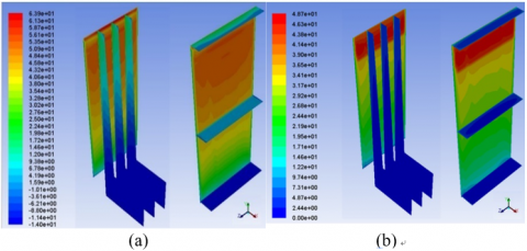
Figure 7. Temperature inside the solar chimney, in centerline section, at 12:30: (a) winter solstice and(b) summer solstice
Table 6. Efficiency of a solar chimney system during the solstices
|
|
21 June |
22 December |
|
η [%] |
0.25 |
0.26 |
Figure 8. Temperature of vertical wall, in centerline section, at 12:30: (a) winter solstice (b) and summer solstice
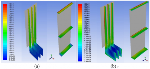
Figure 9. Velocity along the centerline section at 12:30: (a) winter solstice and (b) summer solstice
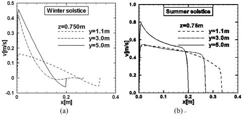
Figure 5 show how the velocity values grow in the channel, near the outlet section, thanks to air heating. At 12:00, when the Sun is in front of the structure, velocity is higher and its maximum value is equal to 0.87 m/s for the 21 June and is equal to 0.98m/s for the other days. Comparing the efficacy of the system between summer and winter solstice (21/06 and 22/12 respectively) at the 12:30 for both days, as shown in the figures 7-11 and in the table 6, it is possible to note that this configuration of solar chimney presents similar performances and similar values of the efficiency. The temperature is been evaluated as a difference between inside-outside of the solar chimney.
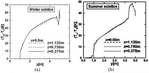
Figure 10. Temperature of vertical wall, of vertical and horizontal planes, at 12:30: (a) winter solstice (a and summer solstice (b)
Figure 11. Velocity along the vertical and horizontal planes, at 12:30 in winter solstice (a) and summer solstice (b)
The next figures represent the profiles of velocity and temperature inside the solar chimney.
For the efficiency, η, it was used this formula:
$η= \frac{\dot{m}∙c_p∙(T_m-T_0)}{G∙S}$ (9)
In the equation 9: “
$\dot{m}$” is the mass flow rate at the outlet section of the solar chimney (kg/s); “cp ” is the specific heat, of the air, at constant pressure and it is equal to 1006.43 J/kg K; “Tm” is the mixing temperature at the outlet section of the solar chimney (K); “ T0” is the external temperature, (K); “G” (W/m2) is the Direct Normal Solar Irradiation and “S” (m2) is the glass surface.In this paper is presented a numerical investigation on a prototypal solar chimney system integrated in a south façade of a building.
The chimney has a converging channel with one vertical aluminum wall and one inclined low-emissivity glass wall.
The analysis is carried out on a three-dimensional model in airflow and the governing equations are given in terms of k-ε turbulence model. The problem is solved by means of the commercial code Ansys-Fluent and the simulations are carried out considering the solar irradiance for assigned geographical location and for a daily distribution during the equinoxes and solstices. Moreover, it was examined and discussed that the heat fluxes vary during the day, so temperature distributions are not uniform: values are lower on the bottom of the wall, because solar rays reach this part more difficultly. Performances are better when heat flux is higher and Sun is in front of chimney.
From the reported profiles of temperature and velocity, it is evident that during the summer solstice the difference of temperature between inside-outside of the chimney is less compared to winter solstice.
It could be interesting, in the future developments, estimate the importance of different type of glass, for best known how this material participates at the phenomenon.
|
I |
radiation intensity, W/m2 |
|
L |
channel high, m |
|
H |
ground distance, m |
|
W |
channel width, m |
|
CP |
specific heat at constant pressure, J/Kg·K |
|
Cε1, Cε2, Cμ |
empirical constants in the k-ε turbulence model |
|
D |
extra term in Eq. 5 |
|
E |
roughness parameter |
|
f1, f2, fμ |
wall damping function |
|
Gb |
production of turbulent kinetic energy due to buoyancy |
|
Gk |
production of turbulent kinetic energy due to buoyancy |
|
hy |
local heat transfer coefficient, W/m2·K |
|
k |
kinetic energy of turbulence |
|
ṁ |
mass flow rate, kg/s |
|
Nuy |
local Nusselt number |
|
$q ̇$ |
heat flux, W/m2 |
|
Prt |
turbulent Prandtl number |
|
To |
ambient temperature, K |
|
Ts |
channel wall (surface) temperature, K |
|
Greek symbols |
|
|
a |
absorbption coefficient, m2/s |
|
b |
thermal expansion coefficient, K-1 |
|
η |
efficiency, % |
|
κ |
thermal conductivity, W/m·K |
|
μ |
laminar viscosity, Pa·s |
|
μt |
turbulent viscosity, Pa·s |
|
ν |
molecular kinematic viscosity, m2/s-1 |
|
σ |
Stefan-Boltzmann constant, W/m2∙K4 |
|
σk |
Prandtl number for k |
|
σε |
Prandtl number for ε |
[1] Haaf W, Friedrich K, Mayer G, Schlaich J. (1983). Solar chimneys Part I: principle and construction of the pilot plant in Manzanares. International Journal of Solar Energy 2: 3-20. https://doi.org/10.1080/01425918308909911
[2] Schlaich J. (1995). The solar chimney: Electricity from the Sun. Eergermann und Partner.
[3] Vieira RS, Petry AP, Rocha LAO, Isoldi LA, dos Santos ED. (2017). Numerical evaluation of a solar chimney geometry for different ground temperatures by means of constructal design. Renewable Energy 109: 222-234. https://doi.org/10.1016/j.renene.2017.03.007
[4] Shirvan KM, Mirzakhanlari S, Mamourian M, Abu-Hamdeh N. (2017). Numerical investigation and sensitivity analysis of effective parameters to obtain potential maximum power output: A case study on Zanjan prototype solar chimney power plant. Energy Conversion and Management 136: 350-360. https://doi.org/10.1016/j.enconman.2016.12.081
[5] Hua SD, Leung DYC, Chan JCY. (2017). Numerical modelling and comparison of the performance of diffuser-type solar chimneys for power generation. Applied Energy 204: 948-957. https://doi.org/10.1016/j.apenergy.2017.03.040
[6] Hua SD, Leung DYC, Chan JCY. (2017). Impact of the geometry of divergent chimneys on the power output of a solar chimney power plant. Energy 120: 1-11. https://doi.org/10.1016/j.energy.2016.12.098
[7] Hua SD, Leung DYC, Chan JCY. (2017). Effect of divergent chimneys on the performance of a solar chimney power plant. Energy Procedia 105: 7-13. https://doi.org/10.1016/j.egypro.2017.03.273
[8] Ayadi A, Driss Z, Bouabidi A, Abid MS. (2017). Experimental and numerical study of the impact of the collector roof inclination on the performance of a solar chimney power plant. Energy and Buildings 139: 263-276. https://doi.org/10.1016/j.enbuild.2017.01.047
[9] Ayadi A, Driss Z, Bouabidi A, Abid MS. (2017). Experimental and numerical analysis of the collector roof height effect on the solar chimney performance. Renewable Energy 115: 649-662. https://doi.org/10.1016/j.renene.2017.08.099
[10] Gholamalizadeh E, Kim MH. (2016). CFD (computational fluid dynamics) analysis of a solar-chimney power plant with inclined collector roof. Energy 107: 661-667. https://doi.org/10.1016/j.energy.2016.04.077
[11] Esfidani MT, Raveshi S, Shahsavari M. (2015). Computational study on design parameters of a solar chimney. International Conference on Sustainable Mobility Applications, Renewables and Technology (SMART). https://doi.org/10.1109/SMART.2015.7399268
[12] Bahar FA, Guellouz MS, Sahraoui M, Kaddeche S. (2015). A numerical study of solar chimney power plants in tunisia. Journal of Physics: Conference Series 596. https://doi.org/10.1088/1742-6596/596/1/012006
[13] Sudprasert S, Chinsorranant C, Rattanadecho P. (2016). Numerical study of vertical solar chimneys with moist air in a hot and humid climate. International Journal of Heat and Mass Transfer 102: 645-656. https://doi.org/10.1016/j.ijheatmasstransfer.2016.06.054
[14] Bianco N, Langellotto L, Manca O, Nardini S. (2010). Radiative effects on natural convection in vertical convergent channels. International Journal of Heat and Mass Transfer 53: 3513-3524. https://doi.org/10.1016/j.ijheatmasstransfer.2010.04.012
[15] Langellotto L, Manca O. (2011). Correlations for natural convection in vertical convergent channels with conductive walls and radiative effects. Heat Transf. Eng 32: 439-454. https://doi.org/10.1080/01457632.2010.506166
[16] Manca O, Nardini S, Ricci D, Tamburrino S. (2011). Numerical study of transient natural convection in air in vertical divergent channels. Numerical Heat Transf., Part A: App 60: 580-603. https://doi.org/10.1080/10407782.2011.616780
[17] Manca O, Nardini S, Romano P, Mihailov E. (2014). Numerical investigation of thermal and fluid dynamic behavior of solar chimney buildings systems. Journal of Chemical Technology and Metallurgy 49: 106-116.
[18] Buonomo B, Manca O, Nardini S, Tartaglione G. (2014). Numerical simulation of convective-radiative heat transfer in a solar chimney. 12th Biennial Conference on Engineering Systems Design and Analysis: 20390. https://doi.org/10.1115/ESDA2014-20390
[19] Buonomo B, Manca O, Montaniero C, Nardini S. (2015). Numerical investigation of convective-radiative heat transfer in a building-integrated solar chimney. Advances in Building Energy Research 9(2): 253-266. https://doi.org/10.1080/17512549.2015.1014840
[20] Cirillo L, Di Ronza D, Fardella V, Manca O, Nardini S. (2015). Numerical and experimental investigations on a solar chimney integrated in a building facade. International Journal of Heat and Technology 33(4): 246-254. https://doi.org/10.18280/ijht.330433
[21] Zha XY, Zhang J, Qin MH. (2017). Experimental and numerical studies of solar chimney for ventilation in low energy buildings. Procedia Engineering 205: 1612-1619. https://doi.org/10.1016/j.proeng.2017.10.294
[22] Coppi M, Quintino A, Salata F. (2013). Numerical study of a vertical channel heated from below to enhance natural ventilation in a residential building. International Journal of Ventilation 12(1): 41-49. https://doi.org/10.1080/14733315.2013.11684001
[23] Montelpare S, D’Alessandro V, Zoppi A, Constanzo E. (2017). A solar chimney for renewable energy production: Thermos-fluid dynamic optimization by CFD analyses. Journal of Physics Conference Series 923(1): 012047. https://doi.org/10.1088/1742-6596/923/1/012047
[24] Bouabidi A, Ayadi A, Nasraoui H, Driss Z, Abid MS. (2018). Study of solar chimney in Tunisia: Effect of the chimney configurations on the local flow characteristics. Energy and Buildings 169: 27-38. https://doi.org/10.1016/j.enbuild.2018.01.049
[25] Al-Kayiem HH, Sreeiaya KV, Chikere AO. (2018). Experimental and numerical analysis of the influence of inlet configuration on the performance of a roof top solar chimney. Energy and Buildings 159: 89-98. https://doi.org/10.1016/j.enbuild.2017.10.063
[26] Hassan A, Ali M, Waqas A. (2018). Numerical investigation on performance of solar chimney power plant by varying collector slope and chimney diverging angle. Energy 142(1): 411-425. https://doi.org/10.1016/j.energy.2017.10.047
[27] Ahmed OK, Hussein AS. (2018). New design of solar chimney (case study). Case Studies in Thermal Engineering 11: 105-112. https://doi.org/10.1016/j.csite.2017.12.008
[28] Buonomo B, Cascetta F, Cirillo L, Manca O, Nardini S. (2018). Thermal and fluid dynamic analysis of a solar chimney integrated in a building façade. International Heat Transfer Conference.
[29] Launder BE, Spalding DB. (1974). The numerical computation of turbulent flow. Computer Methods in Applied Mechanics and Engineering 3: 269-289. https://doi.org/10.1016/0045-7825(74)90029-2
[30] Fluent Inc. (2009). Fluent 6 manuals. Fluent Inc. ed.
[31] Coelho PJ, Carvalho MG. (1997). A conservative formulation of the discrete transfer method. Journal of Heat Transfer 119(1): 118-128. https://doi.org/10.1115/1.2824076
[32] Fluent-Inc. (2007). Gambit 2.4 Modeling Guide ed.
[33] Buonomo B, Cascetta F, Diana A, Manca O, Nardini S. (2019). Numerical investigation on thermal and fluid dynamic analysis of a solar chimney integrated in a building façade. ASME 2019 Summer Heat Transfer Conference.