Khawla Sleiman* | Stefan Van Vaerenbergh | Tayssir Hamieh*
OPEN ACCESS
The physical phenomenon of thermodiffusion is the transfer mechanism that occurs when a thermal gradient is applied to a mixture. It is known as “the Soret |Effect”, of which much experimental and theoretical work has been done to interpret it scientifically. This article briefly presents a one-dimensional theoretical and numerical approach, based on the first law of thermodynamics, of the concentration distribution of the NaCl in a salinity-gradient solar pond. The theoretical developments aim to frame its fluido-thermodynamic factors.
fluid, themodynamic, solar, theoretical
At the turn of the last century, the solar pond was discovered as a “natural phenomenon” in the Transylvanian Medve Lake, in Hungary, where temperatures reaching 70°C were recorded at a depth of 1.32 m, at the end of the summer season; while the minimum temperature was 26°C in early spring. The bottom of this lake containing NaCl salt had a concentration of 26% [1]. This same phenomenon has been observed and reported by others as well [2-7]. Then solar ponds were artificially constructed as large-scale collectors of solar energy, absorbing solar radiation and storing it as thermal energy for long periods of time [8].
In 1948, Block suggested the adoption of a density gradient in the solar pond, to eliminate the convection currents that normally develop in the presence of hot water below cold water. So, a strong density gradient from bottom to top is achieved by using a high concentration of suitable salts at the bottom of the basin and a negligible concentration at the top. Suitable salt should verify the following characteristics: high solubility value to ensure high solution densities, temperature insensitive solubility, sufficiently transparent solution to solar radiation, environmentally friendly salt, safe to handle and available in abundance near the site [9]. The thermal conductivity of saline solution decreases with increasing salinity, and thus acts as an insulating layer. This type of pond is called a “salinity-gradient solar pond SGSP” [1]. The method of generating the salt concentration gradient in the pond can be chosen according to local requirements [10], so it can be done by: natural diffusion, stacking, redistribution or falling.
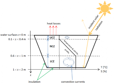
SGSPs, generally 1 to 2 m deep with an isolated base, are made up of three thermally distinct layers [8, 9, 11] (Figure 1):
i) The upper surface layer (0.1-0.4 m) or upper convective zone, whose temperature and salinity are constant, is an area of cooler, less salty water as it forms due to upward transport of salt, surface heating and cooling, and wave action; it supports, therefore, all environmental influences.
ii) The second layer or non-convective zone has temperature and salinity gradients and acts as a critical insulator for the lower zone (where heat will be stored). Its thickness varies from 0.6 to 1.0 m and depends on the desired temperature, solar transmission properties and thermal conductance of water.
iii) The bottom layer, known as lower convective zone or heat-storage zone, is a layer of high salinity brine where temperatures are highest in order to store solar thermal energy efficiently. Useful heat is usually extracted from this layer. Its thickness depends on the temperature and the amount of thermal energy to be stored.
Figure 1. Schematic of salinity-gradient solar pond
In an isotropic fluid system of an enclosed medium with no external forces, concentration gradient builds up due to the driving force of applied temperature gradient until system reaches into the steady state condition [12]. This phenomenon is called “Thermodiffusion or Soret effect”. Because of its popularity, remarkable attention has been focused on the experiments with optical techniques and theoretical models based on non-equilibrium thermodynamics [12].
Thermodiffusion can be studied in a solar pond as a type of top-heated convectionless diffusion medium. The first surface centimeter of the brine absorbs long wavelength radiation (1.2 µm) which forms 22.4% of incoming solar radiation, leading to a sharp increase in the temperature and creating a hot zone in the UCZ. The remaining 77.6% will be distributed to the rest of the pond [13]. The hot zone begins to descend slowly towards the NCZ until it finally reaches the LCZ, as the temperature increases and the pond approaches the pseudo-stationary state. So, the LCZ does not act as the hottest area of the pond from the start. Maintaining the UCZ at a sinusoidal temperature inferior to the temperature of the LCZ eliminates the instabilities, because the density increases in the direction of the gravity field and the fluid will be kept at rest.
3.1 Theoretical approach
Determining the temperature distribution T(z,t) in the pond allows us to find a theoretical approach to understand the phenomenon of thermodiffusion in terms of scientific interpretation. To do this, we use a differential equation whose solution, for prescribed boundary conditions, provides the temperature distribution in the pond.
The one-dimensional partial differential equation describing the distribution of heat is given by [14]:
$\frac{\partial T}{\partial t}\,=\kappa \,\frac{{{\partial }^{2}}T}{\partial {{z}^{2}}}$ (1)
0 < z < L, t > 0.
In Eq. (1), the temperature T is a function of position z and time t, and: $\kappa=\frac{k}{\rho C_{P}}$ is called thermal diffusivity measured in m2/s; where k, r and CP are thermal conductivity, density, and specific heat capacity, respectively.
The initial and boundary conditions are, respectively:
$T\left( z,t=0 \right)={{T}_{init}}\left( z \right)$ (2)
$T\left( z=0,t \right)={{T}_{0}}\left( t \right)$ (3)
$T\left( z=L,t \right)={{T}_{L}}\left( t \right)$ (4)
Suppose no loss of heat from the solar pond surfaces, and the boundary conditions (3) and (4) are, respectively:
${{T}_{0}}\left( t \right)={{T}_{0,av}}+\Delta T\sin \left( \omega t \right)$ (5)
${{T}_{L}}\left( t \right)={{T}_{L}}$ (6)
then, let:
$T=u+w$ (7)
3.1.1 Ends kept at zero temperature and initial temperature f(z)
$\frac{\partial u}{\partial t}\,=\kappa \,\frac{{{\partial }^{2}}u}{\partial {{z}^{2}}}$ (8)
0 < z < L, t > 0.
The initial and boundary conditions are, respectively:
$u\left( z,t=0 \right)=f\left( z \right)$ (9)
$u\left( z=0,t \right)=u\left( z=L,t \right)=0$ (10)
Carslaw and Jaeger [15] presented a simple form of solution of the heat equation, for steady-state temperature oscillations. If the initial temperature is:
$u\left( z=0 \right)=\sum\limits_{n=1}^{\infty }{{{A}_{n}}\sin \left( {{\lambda }_{n}}z \right)}$ (11)
${{\lambda }_{n}}=\frac{n\pi }{L}$ (12)
where, A is the rate of heat production per unit time per volume and ln the eigenvalue, then:
$u\left( z=t \right)=\sum\limits_{n=1}^{\infty }{{{A}_{n}}\sin \left( {{\lambda }_{n}}z \right)}{{e}^{-\kappa \lambda _{n}^{2}t}}$ (13)
will satisfy the conditions (9) and (10) of the problem.
The initial condition (9), supposed as a bounded function satisfying Dirichlet’s conditions, can be expanded in the sine series:
$f\left( z \right)=\sum\limits_{n=1}^{\infty }{{{a}_{n}}\sin \left( {{\lambda }_{n}}z \right)}$ (14)
where,
${{a}_{n}}=\frac{2}{L}\sum\limits_{n=1}^{\infty }{\int\limits_{0}^{L}{f(z)}\sin \left( {{\lambda }_{n}}z \right)}dz$ (15)
So, consider:
$u\left( z=t \right)=\sum\limits_{n=1}^{\infty }{{{a}_{n}}\sin \left( {{\lambda }_{n}}z \right)}{{e}^{-\kappa \lambda _{n}^{2}t}}$ (16)
Continuous function of the two variables z and t, in the regions 0 ≤ z ≤ L and t > 0. $\frac{\partial u}{\partial t}$ and $\kappa \frac{\partial^{2} u}{\partial z^{2}}$ are also uniformly convergent in the intervals of z and t, respectively. So, the Eq. (8) is satisfied at any point of the studied physical system, when t > 0, by the function (16). The initial and boundary conditions, (9) and (10), are also satisfied.
In our physical problem, the initial condition is:
${{T}_{init}}(z)=f(z)=\frac{{{T}_{L}}-{{T}_{0,av}}}{L}z+{{T}_{0,av}}$ (17)
The function (16) becomes:
$u\left( z=t \right)=\sum\limits_{n=1}^{\infty }{\frac{2}{n\pi }\left[ {{T}_{0,av}}-{{\left( -1 \right)}^{n}}{{T}_{L}} \right]\sin \left( {{\lambda }_{n}}z \right){{e}^{-\kappa \lambda _{n}^{2}t}}}$ (18)
This series converges slowly for small values of (kt/L2), say:
$\frac{\kappa t}{{{L}^{2}}}\prec 0.01$ (19)
3.1.2 Ends at variable temperatures and zero initial temperature
$\frac{\partial w}{\partial t}\,=\kappa \,\frac{{{\partial }^{2}}w}{\partial {{z}^{2}}}$ (20)
0 < z < L, t > 0.
The initial and boundary conditions are, respectively:
$w\left( z,t=0 \right)=0$ (21)
$w\left( z=0,t \right)={{T}_{0}}(t)$ (22)
$w\left( z=L,t \right)={{T}_{L}}(t)$ (23)
Duhamel's theorem states that if:
$w=F\left( z,\tau ,t \right)$ (24)
represents the temperature, at position z and time t, of a system with zero initial temperature and surface temperature TS(z,t); then the solution of the problem, in which the initial temperature is zero and the surface temperature is TS(z,t), will be given by:
$w=\int\limits_{0}^{t}{\frac{\partial }{\partial t}F\left( z,\tau ,t-\tau \right)d\tau }$ (25)
Then if:
$w=F\left( z,t \right)$ (26)
represents the temperature, at position z and time t, of a system with zero initial temperature and a surface maintained at unit temperature; then the solution of the problem, when the surface is kept at the temperature TS(t), will be given by:
$w=\int\limits_{0}^{t}{{{T}_{S}}(\tau )\frac{\partial }{\partial t}F\left( z,t-\tau \right)d\tau }$ (27)
Thus, when the surface temperatures are T0(t) and TL(t), we get:
$w=\int\limits_{0}^{t}{\left[ {{T}_{0}}(\tau )\frac{\partial }{\partial t}{{F}_{0}}\left( z,t-\tau \right)+{{T}_{L}}\left( \tau \right)\frac{\partial }{\partial t}{{F}_{L}}\left( z,t-\tau \right) \right]d\tau }$ (28)
where,
${{F}_{0}}\left( z,t-\tau \right)=1-\frac{z}{L}-\frac{2}{\pi }\sum\limits_{n=1}^{\infty }{\frac{1}{n}{{e}^{-\kappa \lambda _{n}^{2}(t-\tau )}}\sin ({{\lambda }_{n}}z)}$ (29)
and:
$F_{L}(z, t-\tau)=\frac{z}{L}+\frac{2}{\pi} \sum_{n=1}^{\infty} \frac{1}{n} e^{-\kappa {\lambda}_{n}^{2}(t-\tau)} \cos (n \pi) \sin \left(\lambda_{n} z\right)$ (30)
By plugging the conditions (5) and (6) in the equation (28), we obtain:
$\begin{align} & w=\sum\limits_{n=1}^{\infty }{\frac{2}{n\pi }[1-{{e}^{-\kappa \lambda _{n}^{2}t}}][{{T}_{0,av}}-{{(-1)}^{n}}{{T}_{L}}]\sin ({{\lambda }_{n}}z)} \\ & +\Delta T\sum\limits_{n=1}^{\infty }{\left[ \frac{2n\pi \kappa \omega {{L}^{2}}}{{{\omega }^{2}}{{L}^{4}}+{{\kappa }^{2}}{{\left( n\pi \right)}^{4}}} \right]} \\ & \left[ \begin{matrix} {{e}^{-\kappa \lambda _{n}^{2}t}}-\cos (\omega t) \\ +\frac{\kappa }{\omega }\lambda _{n}^{2}\sin (\omega t) \\ \end{matrix} \right]\sin ({{\lambda }_{n}}z) \\ \end{align}$ (31)
3.1.3 Temperature distribution
Finally, by inserting (18) and (31) in Eq. (7), we obtain:
$\begin{align} & T(z,t)=\sum\limits_{n=1}^{\infty }{\frac{2}{n\pi }[{{T}_{0,av}}-{{(-1)}^{n}}{{T}_{L}}]\sin ({{\lambda }_{n}}z)} \\ & +\Delta T\sum\limits_{n=1}^{\infty }{\left[ \frac{2n\pi \kappa \omega {{L}^{2}}}{{{\omega }^{2}}{{L}^{4}}+{{\kappa }^{2}}{{\left( n\pi \right)}^{4}}} \right]} \\ & \left[ \begin{matrix} {{e}^{-\kappa \lambda _{n}^{2}t}}-\cos (\omega t) \\ +\frac{\kappa }{\omega }\lambda _{n}^{2}\sin (\omega t) \\ \end{matrix} \right]\sin ({{\lambda }_{n}}z) \\ \end{align}$ (32)
3.2 Approximate form
Carslaw and Jaeger [15] considered the problem of the system 0 < z < L, at zero initial temperature and surfaces z =0 and z = L maintained at T0 = 0 and TL = sin(wt+ε), respectively. The temperature distribution is given by:
$T(z,t)=A\sin (\omega t+\varepsilon +\varphi )+2\pi \kappa \sum\limits_{n=1}^{\infty }{\left[ \frac{n{{(-1)}^{n}}({{n}^{2}}\pi \kappa \sin \varepsilon -\omega {{L}^{2}}\cos \varepsilon )}{{{(\omega L)}^{2}}+{{\kappa }^{2}}{{\left( n\pi \right)}^{4}}} \right]{{e}^{-\kappa \lambda _{n}^{2}t}}\sin ({{\lambda }_{n}}z)}$ (33)
The first term of the temperature function (33) is the steady state periodic solution and the second term is the transient one. The quantities A and Ø are the amplitude and phase of the steady temperature oscillation, at the point z, respectively.
$A=\left| \frac{\sinh [k(1+i)z]}{\sinh [k(1+i)L]} \right|=\sqrt{\frac{\cosh (2kz)-\cos (2kz)}{\cosh (2kL)-\cos (2kL)}}$ (34)
$\varphi =\arg \frac{\sinh [k(1+i)z]}{\sinh [k(1+i)L]}$ (35)
where,
$k=\sqrt{\frac{\omega }{2\kappa }}$ (36)
Then, for the system 0 < z < L, at initial temperature $T_{\text {init }}(z)=\frac{T_{L}-T_{0, a v}}{L} z+T_{0, a v}$ and surfaces z = 0 and z = L held at T0 = T0,av + ΔTsin(wt) and TL, respectively, an approximation is made by assuming that the depth of influence is less than L.
Note that the depth of influence is given by:
$\psi =\sqrt{\frac{2\kappa }{\omega }}$ (37)
The approximation of the temperature distribution (33) is then:
${{T}_{a}}(z,t)={{T}_{init}}(z)+{{A}_{a}}(z)\Delta T\sin [\omega t+{{\varphi }_{a}}(z)]$ (38)
where, Aa, the limit of A, if ψ tends to zero, is supposed to be:
${{A}_{a}}(z)={{e}^{-kz}}$ (39)
and φa, the linear approximation of φ so that A does not vanish, is:
${{\varphi }_{a}}(z)=-kz$ (40)
The solution (38) does not contain any series. It will be valid if t is greater than the period of oscillation: t > (1/w), and applicable for long-term average mass flux. It should work well if L > 10 ψ. For a thermal diffusivity of water k = 10-7 m2/s and a pulsation w = 7.27×10⁻⁵ Hz (for a period T of 24 hours), the depth of influence ψ = 0.05 m. Hence, the approximation is valid for a depth L > 0.5 m, let L = 1 m in our problem.
3.3 ‘Mathematica’ form
For the initial and boundary conditions (17), (5) and (6), respectively, the temperature distribution is given by ‘Mathematica’ as follow:
$T(z, t)=T_{0, a v}+\Delta T \sin (\omega t) \\ -\frac{z}{L}\left[T_{0, a v}+\Delta T \sin (\omega t)-T_{L}\right] \\ \frac{2}{\lambda_{n}^{2}}\left[\frac{\omega \sin (n \pi)-n \pi \omega}{\omega^{2} L^{4}+\kappa^{2}(n \pi)^{4}}\right] \\ +\Delta T \sum_{n=1}^{\infty}\left[\begin{array}{c}(n \pi)^{2} \kappa \cos (\omega t) \\ +\omega L^{2} \sin (\omega t) \\ -(n \pi)^{2} \kappa e^{-\kappa \lambda_{n}^{2} t}\end{array}\right] \\ \times \sin \left(\lambda_{n} z\right)$ (41)
Diffusion of matter is the transfer, by random molecular motions, of mass resulting from concentration differences of one or more constituents of a mixture, without convective movement. Consequently, we can only have diffusion if at least two distinct species are present. The constituents of an initially uniform mixture are liable to separate – on the molecular level – when this mixture is subjected to a temperature gradient [16]. The analogy between the heat diffusion – which is also due to random molecular motions – and the diffusion of matter, first recognized by Fick, in 1855, led him to put the diffusion of matter on a quantitative basis using the heat diffusion mathematical equation of Fourier, in 1822 [17]. Then, the mathematical theory of mass diffusion in isotropic substances is:
$F=-D\frac{\partial c}{\partial z}$ (42)
where F is the rate of transfer per unit area of section.
The fundamental differential equation of diffusion in an isotropic medium is derived from the equation (42):
$\frac{\partial c}{\partial z}=D\frac{{{\partial }^{2}}c}{\partial {{z}^{2}}}$ (43)
Due to the mass conservation, there is only one independent component of a binary mixture [16]. The mass fraction of the independent component, which is the solute, is denoted as c. So, the mass fraction of the dependent component, which is the solvent, will be 1 – c.
In presence of temperature gradient, the expression of the mass flow of the independent component is given by:
$J=-\rho \left( D\frac{{{\partial }^{2}}c}{\partial {{z}^{2}}}+{{D}_{T}}\frac{{{\partial }^{2}}T}{\partial {{z}^{2}}} \right)$ (44)
Thermodiffusion processes are quantified by mass and thermodiffuison coefficients, D and DT, respectively. The thermodiffusion coefficient can be written as:
$\mathrm{D}_{\mathrm{T}}=\mathrm{D} \times \mathrm{S}_{\mathrm{T}}$ (45)
where, ST is the Soret coefficient.
With no flow and in a transient mode, the problem will be one-dimensional and the concentration gradient expressed in the following form:
$\frac{\partial c}{\partial t}=D\frac{{{\partial }^{2}}c}{\partial {{z}^{2}}}+F(z,t)$ (46)
0 < z < L, t > 0.
where,
$F(z,t)={{D}_{T}}\frac{{{\partial }^{2}}T}{\partial {{z}^{2}}}$ (47)
Let the concentration c at the end z = L, in other words at the lower convective zone:
c(z = L, t) = cL = 0.25 (48)
At z = 0, in the upper convective zone where water is less salty, the concentration is much lower than cL. Then:
c(z = 0, t) = c0 ≈ 0 (49)
The initial condition is thus:
$c(z,t=0)={{c}_{init}}(z)=\frac{{{c}_{L}}-{{c}_{0}}}{L}z+{{c}_{0}}=\frac{{{c}_{L}}}{L}z$ (50)
For this nonhomogeneous problem, suppose that:
$v(z,t)=c(z,t)-\frac{{{c}_{L}}}{L}z$ (51)
The problem becomes:
$\frac{\partial v}{\partial t}=D\frac{{{\partial }^{2}}v}{\partial {{z}^{2}}}+F(z,t)$ (52)
0 < z < L, t > 0
with initial and boundary conditions, respectively:
v(z, 0) = 0 (53)
v(0, t) = v(L, t) = 0 (54)
4.1 Using the temperature distribution (32)
Relation (47) can be expressed as follow:
$F(z,t)=\sum\limits_{n=1}^{\infty }{{{F}_{n}}(t)\sin ({{\lambda }_{n}}z)}$ (55)
Then:
${{F}_{n}}(t)=\frac{2}{L}\sum\limits_{n=1}^{\infty }{\int\limits_{0}^{L}{F(z,t)\sin ({{\lambda }_{n}}z)dz}}$ (56)
and v(z, t) expressed as follow:
$v(z,t)=\sum\limits_{n=1}^{\infty }{{{G}_{n}}(t)\sin ({{\lambda }_{n}}z)}$ (57)
Then, by plugging the expressions (55) and (57) in the equation (52), we obtain:
$\sum\limits_{n=1}^{\infty }{\left[ \frac{d{{G}_{n}}}{dt}-D\lambda _{n}^{2}{{G}_{n}} \right]=\sum\limits_{n=1}^{\infty }{{{F}_{n}}}}$ (58)
where Gn will be expressed as:
${{G}_{n}}(t)=\sum\limits_{n=1}^{\infty }{{{e}^{-D\lambda _{n}^{2}t}}\int\limits_{0}^{t}{{{F}_{n}}(\tau ){{e}^{D\lambda _{n}^{2}\tau }}d\tau }}$ (59)
By plugging the expression (32) of the temperature in the Eq. (56), we obtain:
$\begin{align} & c(z,t)=\frac{{{c}_{L}}}{L}z-{{D}_{T}}\sum\limits_{n=1}^{\infty }{\sin ({{\lambda }_{n}}z)} \\ & \times \left\{ \begin{matrix} \frac{2}{n\pi D}\left[ {{T}_{0,av}}-{{(-1)}^{n}}{{T}_{L}} \right]\left[ 1-{{e}^{-D\lambda _{n}^{2}t}} \right] \\ +\frac{{{B}_{n}}}{D-\kappa }\Delta T\left[ {{e}^{-\kappa \lambda _{n}^{2}t}}-{{e}^{-D\lambda _{n}^{2}t}} \right] \\ -{{B}_{n}}{{C}_{n}}\lambda _{n}^{2}\Delta T\left[ \sin (\omega t)-\frac{D}{\omega }\lambda _{n}^{2}{{e}^{-D\lambda _{n}^{2}t}}+\frac{D}{\omega }\lambda _{n}^{2}\cos (\omega t) \right] \\ +{{B}_{n}}{{C}_{n}}\lambda _{n}^{4}\Delta T\left( \frac{\kappa }{\omega } \right)\left[ {{e}^{-D\lambda _{n}^{2}t}}-\cos (\omega t)+\frac{D}{\omega }\lambda _{n}^{2}\sin (\omega t) \right] \\ \end{matrix} \right\} \\ \end{align}$ (60)
${{B}_{n}}=\frac{2n\pi \kappa \omega {{L}^{2}}}{{{\omega }^{2}}{{L}^{4}}+{{\kappa }^{2}}{{(n\pi )}^{4}}}$ (61)
${{C}_{n}}=\frac{\omega {{L}^{4}}}{{{\omega }^{2}}{{L}^{4}}+{{D}^{2}}{{(n\pi )}^{4}}}$ (62)
4.2 Using the approximate temperature (38)
The approximate solution (38) of the temperature leads us to a thermodiffusion equation having series of solutions which converge slowly, thus requiring no less than 100 summation terms (N ≥ 100) for stable results. Using ‘Mathematica’, we get the following approximate expression:
$\begin{align} & {{c}_{a}}(z,t)=\frac{{{c}_{L}}}{L}z+\sum\limits_{n=1}^{N}{{{D}_{n}}\sin ({{\lambda }_{n}}z)} \\ & \times \left\{ \begin{matrix} {{E}_{n}}{{e}^{-D\lambda _{n}^{2}t}}-{{E}_{n}}\cos (\omega t)+{{F}_{n}}\sin (\omega t) \\ +{{(-1)}^{n}}{{e}^{-\frac{L}{\psi }}}\left\{ \begin{matrix} \left[ {{E}_{n}}\cos (\omega t)-{{F}_{n}}\sin (\omega t) \right]\cos \left( \frac{L}{\psi } \right) \\ +\left[ {{E}_{n}}\sin (\omega t)+{{F}_{n}}\cos (\omega t) \right]\sin \left( \frac{L}{\psi } \right) \\ \end{matrix} \right\} \\ -{{(-1)}^{n}}{{e}^{-D\lambda _{n}^{2}t-\frac{L}{\psi }}}\left[ {{E}_{n}}\cos \left( \frac{L}{\psi } \right)+{{F}_{n}}\sin \left( \frac{L}{\psi } \right) \right] \\ \end{matrix} \right\} \\ \end{align}$ (63)
$\begin{align} & {{D}_{n}}= \\ & \frac{8n\pi {{L}^{2}}{{D}_{T}}\Delta T}{4{{\omega }^{2}}{{L}^{8}}+{{D}^{2}}{{\psi }^{4}}{{(n\pi )}^{8}}+{{(n\pi L)}^{4}}({{\omega }^{2}}{{\psi }^{4}}+4{{D}^{2}})} \\ \end{align}$ (64)
${{E}_{n}}=\omega {{L}^{4}}-\frac{D{{\psi }^{2}}{{(n\pi )}^{4}}}{2}$ (65)
${{F}_{n}}=\frac{(\omega {{\psi }^{2}}+2D){{(n\pi L)}^{2}}}{2}$ (66)
And as mentioned in equation (37): $\psi=\sqrt{\frac{2 \kappa}{\omega}}$.
4.3 Using the ‘Mathematica’ temperature (41)
By plugging the expression (41) of the temperature in the Eq. (56), we obtain:
$\begin{align} & c(z,t)=\frac{{{c}_{L}}}{L}z-2{{D}_{T}}\Delta T\sum\limits_{n=1}^{\infty }{{{I}_{n}}\sin ({{\lambda }_{n}}z)} \\ & \times \left\{ \begin{matrix} {{J}_{n}}\left[ \sin (\omega t)+\frac{D}{\omega }\lambda _{n}^{2}\cos (\omega t)-\frac{D}{\omega }\lambda _{n}^{2}{{e}^{-D\lambda _{n}^{2t}}} \right] \\ +{{Q}_{n}}\left[ 1-\cos (\omega t)+\frac{D}{\omega }\lambda _{n}^{2}\sin (\omega t) \right] \\ -\frac{\kappa {{L}^{2}}}{D-\kappa }\left[ {{e}^{-\kappa \lambda _{n}^{2t}}}-{{e}^{-D\lambda _{n}^{2t}}} \right] \\ \end{matrix} \right\} \\ \end{align}$ (67)
${{I}_{n}}=\frac{\omega \left[ \sin (n\pi )-n\pi \right]}{{{\omega }^{2}}{{L}^{4}}+{{\kappa }^{2}}{{(n\pi )}^{4}}}$ (68)
${{J}_{n}}=\frac{\kappa \omega {{(n\pi )}^{2}}{{L}^{4}}}{{{\omega }^{2}}{{L}^{4}}+{{D}^{2}}{{(n\pi )}^{4}}}$ (69)
${{Q}_{n}}=\frac{{{\omega }^{2}}{{L}^{6}}}{{{\omega }^{2}}{{L}^{4}}+{{D}^{2}}{{(n\pi )}^{4}}}$ (70)
5.1 Temperature distribution
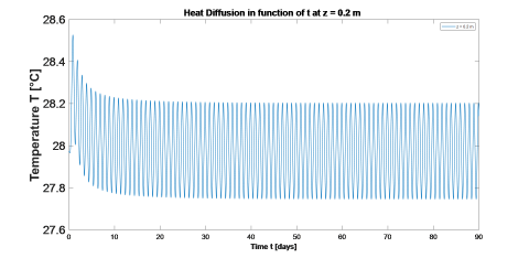
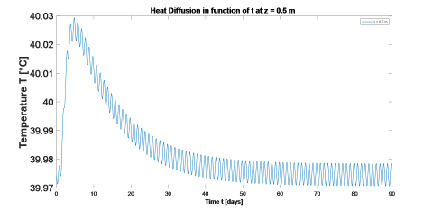
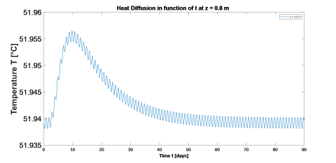
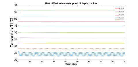
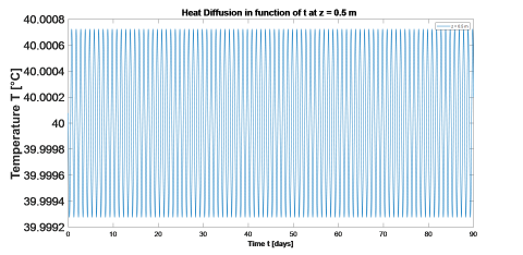
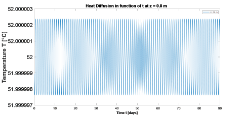
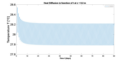
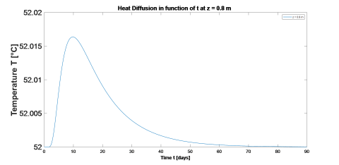
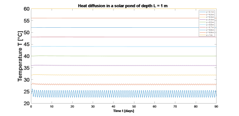
We present here a collection of graphical representation of the temperature distribution in function of time, for different positions in the solar pond. Let the pulsation w = 7.27×10⁻⁵ Hz, water thermal diffusivity k = 10-7 m2/s, pond’s depth L = 1 m, temperature of the bottom (z = L) TL = 60°C, T0,av = 20°C and difference between daily and night temperature ΔT = 10°C.
5.1.1 Theoretical approach, equation (32)
Figure 2. Temperature variation in function of time at a depth z = 0.2 m (UCZ)
Figure 3. Temperature variation in function of time at a depth z = 0.5 m (NCZ)
Figure 4. Temperature variation in function of time at a depth z = 0.8 m (LCZ)
Figure 5. Temperature variation in function of time at different positions z of a 1 m depth solar pond
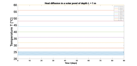
5.1.2 Approximate form, equation (38)
Figure 6. Temperature variation in function of time at z = 0.2 m
Figure 7. Temperature variation in function of time at z = 0.5 m
Figure 8. Temperature variation in function of time at z = 0.8 m
Figure 9. Temperature variation in function of time at different positions z of a 1 m depth solar pond
5.1.3 ‘Mathematica’ form, equation (41)
Figure 10. Temperature variation in function of time at z = 0.2 m
Figure 11. Temperature variation in function of time at z = 0.5 m
Figure 12. Temperature variation in function of time at z = 0.8 m
Figure 13. Temperature variation in function of time at different positions z of a 1 m depth solar pond
5.2 Mass fraction distribution
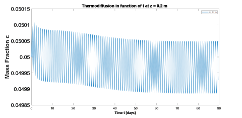
We present here a collection of graphical representation of the mass fraction distribution in function of time, for different positions in the solar pond. Let the diffusion coefficient of NaCl in water D = 10-9 m2/s, thermodiffusion coefficient DT = 10-11 m2/s and mass fraction of the bottom cL = 0.25.
5.2.1 Based on the theoretical approach, equation (60)
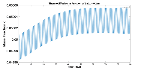
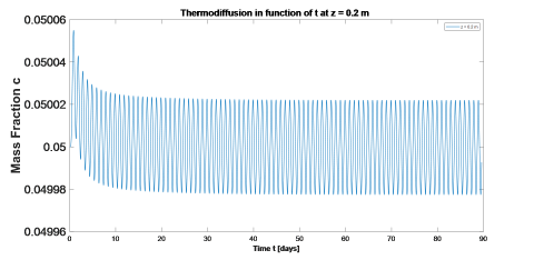
Figure 14. Mass fraction variation in function of time at z = 0.2 m
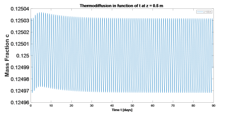
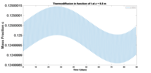
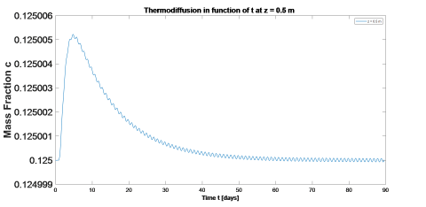
Figure 15. Mass fraction variation in function of time at z = 0.5 m
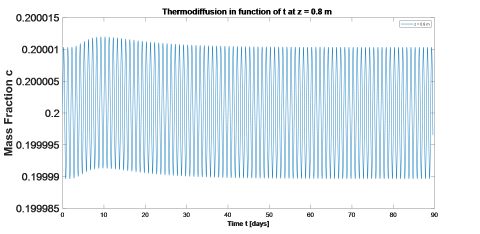
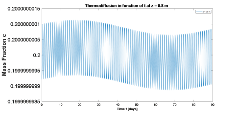
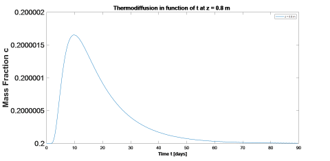
Figure 16. Mass fraction variation in function of time at z = 0.8 m
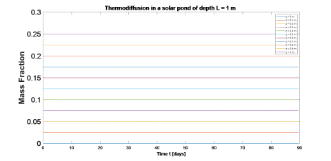
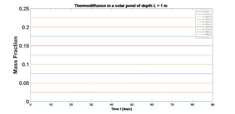
Figure 17. Mass fraction variation in function of time at different positions z of a 1 m depth solar pond
5.2.2 Based on the approximate temperature, equation (63)
Figure 18. Mass fraction variation in function of time at z = 0.2 m
Figure 19. Mass fraction variation in function of time at z = 0.5 m
Figure 20. Mass fraction variation in function of time at z = 0.8 m
Figure 21. Mass fraction variation in function of time at different positions z of a 1 m depth solar pond
5.2.3 Based on ‘Mathematica’ form, equation (67)
Figure 22. Mass fraction variation in function of time at z = 0.2 m
Figure 23. Mass fraction variation in function of time at z = 0.5 m
Figure 24. Mass fraction variation in function of time at z = 0.8 m
Figure 25. Mass fraction variation in function of time at different positions z of a 1 m depth solar pond
In this work, we derived one-dimensional analytical forms describing the variation over time of the mass fraction of the solute, NaCl, along the 3 layers of a salinity gradient solar pond. A small pond of 1 m depth was considered. The model involved two initial conditions and four boundary conditions, for the temperature and the mass fraction, where the surface temperature was sinusoidal in function of time. The computed results show that the boundary sinusoidal temperature leads to a sinusoidal variation of the mass fraction in function of time all along the pond. These results should be compared with experimental data taken from a pond which we aim to build in Lebanon to verify our analytical forms and match parameters and factors.
|
A |
Rate of heat production per unit time per volume |
|
c |
mass fraction of NaCl |
|
c0 cinit |
mass fraction at the surface of the pond mass fraction at t = 0 |
|
cL |
mass fraction at the bottom of the pond |
|
Cp |
specific heat capacity, J.kg-1.°C-1 |
|
D |
diffusion coefficient of NaCl in water, m2/s |
|
DT |
thermodiffusion coefficient, m2/s |
|
F |
rate of transfer per unit area |
|
J |
mass flow of the NaCl, kg/s |
|
k |
thermal conductivity, W.m-1.°C-1 |
|
L |
solar pond height measured from the top, m |
|
n |
summation terms |
|
S |
salinity, % |
|
ST |
Soret coefficient, dimensionless |
|
t |
time, s |
|
T |
temperature, °C |
|
T0 |
temperature of the surface z = 0, °C |
|
Tinit |
initial temperature, at t = 0, °C |
|
TL |
temperature of the bottom z = L, °C |
|
ΔT |
difference between daily and night temperatures, °C |
|
Greek symbols |
|
|
$\kappa$ |
thermal diffusivity, m2. s-1 |
|
$\lambda_{\mathrm{n}}$ |
eigenvalue |
|
$\rho$ |
density, kg.m-3 |
|
$\psi$ |
depth of influence, m |
|
$\omega$ |
pulsation, Hz |
|
Subscripts |
|
|
av |
average |
|
LCZ |
lower convective zone |
|
NCZ |
non-convective zone |
|
SGSP |
salinity-gradient solar pond |
|
UCZ |
upper convective zone |
[1] Khallaf, A.M. (2011). History of the solar ponds: A review study. Renewable and Sustainable Energy Reviews, 15: 3319-3325. https://doi.org/10.1016/j.rser.2011.04.008
[2] Anderson, G.C. (1958). Some limnological features of a shallow saline meromictic lake. Limnology and Oceanography, 3(3): 259-270. https://doi.org/10.4319/lo.1958.3.3.0259
[3] Wilson, A., Wellman, H. (1962). Lake Vanda: An Antarctic lake: Lake Vanda as a solar energy trap. Nature, 196: 1171-1173. https://doi.org/10.1038/1961171a0
[4] Hoare, R.A. (1966). Problems of heat transfer in Lake Vanda. Nature, 210: 787-789. https://doi.org/10.1038/210787a0
[5] Por, F.D. (1970). Solar lake on the shore of the Red-Sea. Nature, 218: 860-861. https://doi.org/10.1038/218860a0
[6] Melack, J.M., Kilham, P. (1972). Lake Mahega: A Mesotropic Sulfactochloride Lake in western Uganda, Afr J Trop Hydro boil Fish, 2(2): 141-150.
[7] Hudica, P.P., Sonnefeld, P. (1974). Hot Brines on Los Roques, Venezuela. Science, 185: 440-442. https://doi.org/10.1126/science.185.4149.440
[8] Suárez, F., et al. (2010). A fully coupled, transient double-diffusive convective model for salt-gradient solar ponds. International Journal of Heat and Mass Transfer, 53(9): 1718-1730. https://doi.org/10.1016/j.ijheatmasstransfer.2010.01.017
[9] Garg, H.P. (1987). Solar ponds. Advances in Solar Energy Technology, Vol. I. D Reidel Publishing Company, Dordrecht, Holland, pp, 259-305. https://doi.org/10.1007/978-94-017-0659-9
[10] Kaushika, N.D. (1948). Solar ponds: A review. Energy Convers Manage, 24(4): 353-376. https://doi.org/10.1016/0196-8904(84)90016-5
[11] Monjezi, A.A., Campbell, A.N. (2016). A comprehensive transient model for the prediction of the temperature distribution in a solar pond under Mediterranean conditions. Solar Energy, 135: 297-307. https://doi.org/10.1016/j.solener.2016.06.011
[12] Rahman, M.A., Saghir, M.Z. (2014). Thermodiffusion or Soret effect: Historical teview. International Journal of Heat and Mass Transfer, 73: 693-705. https://doi.org/10.1016/j.ijheatmasstransfer.2014.02.057
[13] Rabl, A. (1975). Solar ponds for space heating. Solar Energy, 17(1): 1-12. DOI: 10.1016/0038-092X(75)90011-0
[14] Kolodner, P., Williams, H., Moe, C. (1988). Optical measurement of the Soret coefficient of ethanol/water solutions. J Chem Phys, 88(10): 6512. https://doi.org/10.1063/1.454436
[15] Carslaw, H., Jaeger, J. (1959). Linear flow of heat in the solid bounded by two parallel planes. Conduction of Heat in Solids, Clarendon Press, Oxford, London, pp. 92-132.
[16] Mialdun, A., Yasnou, V., Shevtsova, V. (2012). A comprehensive study of diffusion, thermodiffusion, and soret coefficients of water-isopropanol mixtures. J Chem Phys, 136(24). https://doi.org/10.1063/1.4730306
[17] Crank, J. (1975). The diffusion equations. The Mathematics of Diffusion, Clarendon Press, Oxford, London, pp. 1-10.