Dedy Juliandri Panjaitan*![]() | Firmansyah
| Firmansyah![]() | Herman Mawengkang
| Herman Mawengkang![]() | Devy Mathelinea
| Devy Mathelinea![]()
© 2025 The authors. This article is published by IIETA and is licensed under the CC BY 4.0 license (http://creativecommons.org/licenses/by/4.0/).
OPEN ACCESS
Perishable-input industries such as fish processing require production plans that minimize cost, waste, and unmet demand amid volatile markets. We cast this task as a mixed-integer nonlinear programming (MINLP) model that embeds freshness windows, labor-capacity ceilings, and stochastic demand across multiple products and periods. To solve the resulting non-convex problem, we design an enhanced Generalised Reduced Gradient (GRG) algorithm—a projection-based gradient method that activates only locally binding constraints and rounds each iterate to the nearest mixed-integer feasible point, speeding convergence. Tested on an Indonesian plant with eight products over four periods, the MINLP–GRG approach cuts total cost by 5.2% versus classical GRG and 2.1% against a commercial mixed-integer linear programming (MILP) solver, reduces spoilage from 8.1% to 3.2% (≈ 60%), and lowers under-delivery by 45.6%, all within 15 s on a standard workstation. A larger case (20 products, eight periods) converges in 78 iterations (< 62 s) with linear memory growth, showing scalability. The proposed framework therefore delivers measurable economic and sustainability gains for fish-processing operations.
fish processing planning, generalized reduced gradient, mixed-integer nonlinear programming, optimization, production planning, perishable inventory management
Indonesia’s marine-based economy relies heavily on fish processing [1], yet the raw materials sustaining this sector deteriorate almost immediately after harvest [2]. Spoilage erodes profit margins, disrupts supply-chain rhythm [3], and undermines sustainability goals, compelling processors to strike a careful balance between meeting volatile demand and avoiding waste. Effective production planning therefore hinges on models that treat fish as a time-sensitive resource rather than as non-degrading inventory [4], allowing freshness constraints to shape scheduling, procurement, and workforce decisions in an integrated manner [5].
Perishability also magnifies classic planning trade-offs: Inventory held too long invites quality loss and price markdowns [6], whereas underproduction precipitates costly emergency purchases and lost sales [7]. Although a growing body of research explores production planning in agri-food contexts [6], most mixed-integer and economic-order-quantity frameworks assume infinite shelf life, rely on highly simplified decay functions, or focus on single-product settings. These approaches typically overlook how labour availability, resource coupling (e.g., cold-storage capacity), and batch-dependent processing times jointly influence daily scheduling decisions [8], factors that become pivotal when multiple fish products compete for short-lived raw materials inside a dynamic plant environment [9].
To address these shortcomings, the present study develops a mixed-integer nonlinear programming formulation for multi-product fish production planning that explicitly embeds shelf-life-driven flow constraints [4], links production decisions to labour and supplementary-resource requirements [10], and permits economically justified under-delivery or limited carry-over [11]. The resulting model is large, non-convex, and tightly constrained, prompting the design of an enhanced Generalised Reduced Gradient (GRG) algorithm that blends adaptive constraint activation, dynamic step-size adjustment, and a warm-start mechanism to exploit structural similarity across planning periods. This algorithmic design accelerates convergence while safeguarding feasibility under stringent freshness windows.
The research pursues three intertwined objectives: minimising total operational cost while explicitly penalising spoilage, maintaining prescribed service levels in the face of stochastic, multi-period demand, and quantifying how alternative workforce and resource strategies mediate the trade-off between cost efficiency and product freshness.
Building on these objectives, the study delivers four key contributions. First, it offers the first unified optimisation framework that simultaneously captures perishability, multi-product scheduling, and labour–resource coordination within a single tractable model. Second, it advances solution methodology by tailoring an enhanced GRG algorithm to the distinctive structure of perishable production systems, demonstrating how constraint-activation and warm-start strategies can be systematically integrated into gradient-based optimisation. Third, it extends managerial insight by revealing the operational levers. such as cross-trained labour pools and flexible cold-storage allocation, that most effectively balance freshness and cost in fish-processing plants. Finally, it establishes a transferable modelling template that can be adapted to other agri-food sectors where rapid quality decay, multi-product competition, and resource coupling generate similarly complex planning environments.
The concept of perishability profoundly influences inventory management decisions, especially in sectors like fresh fish production where every hour of storage erodes value and narrows processing options. The deterioration of perishable goods imposes a challenge that demands synchronized inventory, production, and pricing decisions with remaining shelf-life. As highlighted in various studies [12-17], failing to model this deterioration explicitly can lead to under- or over-production, hidden waste costs, and declining product quality. Classical Economic Order Quantity (EOQ) models have long framed inventory problems, adapting to include age-, stock-, and price-dependent demand along with back-ordering mechanisms [18, 19]. These EOQ-based approaches typically rely on exponential deterioration functions, yet their steady-state assumptions and single-product focus limit their relevance for dynamic, multi-product environments like fish plants with stochastic demand cycles.
Several EOQ models have been proposed to accommodate the challenges of deterioration. For instance, Fujiwara and Perera [18] introduced exponential penalty cost functions for deteriorating products, while Mashud [20] emphasized fully backlogged shortages under demand-dependent deterioration. Similarly, [19] accounted for demand rates as functions of product age, and [21] modelled fixed-lifetime perishables with full backorders. Further contributions in references [22, 23] examined price and stock-dependent demand in remanufacturing contexts and fuzzy random environments under trade credit regimes, respectively. These studies reinforce that inventory strategies, age-dependent ordering decisions, and issuing rules are intimately tied to perishability dynamics. According to the study by Chen et al. [24], perishable models fall into three broad categories: those with expiration dates, those influenced by storage conditions [25], and those with deterioration rates dependent on random failures [26].
Yet modern applications demand richer models. Contemporary contributions embed perishability within broader supply-chain and production-routing formulations, such as two-stage blood-supply networks, inventory-location-routing with Lagrangian relaxation, and fuzzy multi-objective meat distribution systems—all of which expand problem size and non-linearity [27]. However, these models often resort to metaheuristics that trade off optimality, or general-purpose global solvers that become computationally burdensome with the addition of binary workforce or resource constraints. For instance, Li and Teng [28] modelled freshness-dependent demand where customer preference for longer sell-by dates influences purchasing behaviour, thus shaping dynamic demand curves that rise, stabilize, and fall over a product’s lifecycle.
Perishable inventory management is further complicated by uncertainty in both product quality and client demand, demanding the incorporation of product quality as an optimization criterion alongside stock levels and shipping costs. Kumar et al. [29] emphasized the need to forecast customer behaviour to maintain supply availability and pricing strategies, while Yang et al. [30] proposed a quality-based pricing strategy supported by deep reinforcement learning to ensure buyers are informed about product quality. Recent studies have advanced inventory modeling under dynamic demand conditions, incorporating price-sensitive demand and backorder considerations within a finite planning horizon [31]. This aligns with our focus on perishability-driven replenishment and demand responsiveness, providing a theoretical foundation for integrating cost and service-level objectives in our model. Further, supply chain models are evolving toward sustainability goals. Burgess et al. [32] combined forward and reverse logistics under demand uncertainty and optimized both cost and CO₂ emissions using ant colony algorithms. Cao et al. [33] presented a mathematical model for multi-product perishable supply chains using genetic algorithms for large-scale problem solving. In a similar direction, Rad and Nahavandi [34] developed a green, closed-loop supply chain network that considers supplier discounts and product quality to jointly reduce costs, lower environmental impact, and improve consumer satisfaction.
To handle such complexity with high fidelity, Mixed-Integer Nonlinear Programming (MINLP) emerges as a suitable framework. While generic MINLP solution methods—such as direct-search or branch-and-bound hybrids—have been proposed, they struggle with sparse Jacobians interspersed with repeated dense substructures typical of horizon-coupled, multi-product schedules [35]. The GRG algorithm becomes an attractive alternative, offering a projection-based approach that separates smooth spoilage dynamics from discrete decisions like hiring or lay-offs. Though GRG has been adapted for integer variables using integer line-search strategies [36], no existing studies have tailored it to multi-product perishability-driven production planning problems.
This study fills that gap. We propose a large-scale MINLP model that integrates freshness-window constraints with labour and auxiliary resource planning for eight fish products across four quarterly periods. Our enhanced GRG method embeds dynamic constraint activation, scenario-based warm starts, and integer line-search mechanisms. By leveraging the repetitive block structure inherent in perishable production systems and decomposing the problem using GRG’s natural formulation, the method achieves fast convergence on real data, reducing both spoilage and total cost compared to global solvers. As such, this work extends GRG from a generic nonlinear optimization tool to a tailored engine for perishable-goods scheduling, offering a blueprint for broader agri-food applications where deterioration and resource coupling are central concerns.
An iterative optimization approach called the Generalized Reduced Gradient (GRG) Method is utilized to resolve nonlinear programming issues. In particular, it is meant to tackle convex or quasi-convex problems with differentiable objective function and constraints.
The GRG method is based on the idea of reducing the gradient of the objective function while satisfying the constraints of the problem. The algorithm works by starting at an initial feasible solution and then iteratively improving the solution by finding a direction that reduces the objective function while satisfying the constraints. This direction is found using a gradient-based search.
At each iteration, the GRG method determines whether the current solution is feasible or not. If it is not feasible, the algorithm calculates a new direction that satisfies the constraints and reduces the objective function. If the solution is feasible, the algorithm calculates the gradient of the objective function and checks whether it is close to zero. If the gradient is close to zero, the algorithm terminates and returns the current solution as the optimal solution.
The GRG method is known for its ability to handle complex nonlinear programming problems with many variables and constraints. However, it is sensitive to the initial solution, and it may converge to a local minimum rather than the global minimum. Therefore, multiple runs with different initial solutions may be required to obtain the global minimum. Overall, the GRG method is a powerful tool for solving nonlinear programming problems, and it is widely used in engineering, finance, and other fields.
Building on the classical GRG framework, we embed three mutually reinforcing mechanisms that tailor the search to the perishability and stochasticity of multi-product fish production. First, freshness windows and time-dependent deterioration coefficients are encoded directly in the constraint system, so every projected gradient step is evaluated against explicit shelf-life limits. Second, the line-search routine employs an adaptive step size updated via scenario-based learning: information gleaned from the ensemble of demand scenarios guides step lengths toward regions that historically yield feasible, low-cost solutions, accelerating convergence under uncertainty. Third, to respect discrete labour and capacity decisions, each real-valued iterate is projected onto the nearest mixed-integer point through a rounding-and-refinement procedure that exploits the superbasic structure of the reduced gradient, thereby preserving gradient information while ensuring feasibility. Together, these innovations enable the enhanced GRG algorithm to traverse the feasible region more economically than its standard counterpart while remaining sensitive to perishability, demand variability, and mixed-integer resource constraints.
The GRG method is an iterative optimization algorithm used to solve nonlinear programming problems. The algorithm can be described as follows:
1) Start with an initial feasible solution $x_0$.
2) Compute the gradient of the objective function $f(x)$ and the Jacobian matrix $J(x)$ of the constraints at $x_0$.
3) Solve the system of equations $J\left(x_0\right)^* d=-f^{\prime}\left(x_0\right)$, where $d$ is the direction of descent.
4) Compute the step size $t$ such that $x_1=x_0+t^* d$ is feasible.
5) If $x_1$ is not feasible, find a feasible point $x^{\prime}$ on the line between $x_0$ and $x_1$, and set $x_1=x^{\prime}$.
6) Compute the gradient of the objective function and the Jacobian matrix of the constraints at $x_1$.
7) If the gradient is small enough, terminate and return $x_1$ as the optimal solution. Otherwise, go to step 3 with $x_1$ as the new starting point.
The GRG method works by iteratively improving the solution by finding a descent direction that reduces the objective function while satisfying the constraints. At each iteration, the algorithm checks if the current solution is feasible or not, and if not, it computes a new direction that satisfies the constraints and reduces the objective function. The algorithm terminates when the gradient of the objective function is close to zero, indicating that the current solution is optimal.
To accommodate the operational realities of multi-product fish processing, the classical GRG loop is augmented at three critical junctures. During the Jacobian/gradient evaluation (Step 3) we incorporate time-indexed freshness windows and deterioration coefficients, thereby ensuring that every reduced-space search direction already respects perishability constraints. In the line-search phase (Step 4) the trial step length is adapted through a scenario-learning rule that exploits historical demand realisations to accelerate convergence under uncertainty without sacrificing feasibility. Finally, after the feasibility-restoration step (Step 5) each continuous iterate is projected onto the nearest admissible mixed-integer point and refined via a superbasic update, which preserves descent information while enforcing discrete labour and capacity limits. These targeted modifications allow the enhanced GRG algorithm to navigate the feasible region more efficiently than its standard counterpart while remaining sensitive to perishability, stochastic demand, and mixed-integer resource constraints that characterise real-world fish-production planning.
It is important to remember that the GRG approach might converge to a local minimum as opposed to the global minimum and that it can be sensitive to the starting solution. Therefore, in order to get the global minimum, it might be necessary to perform several runs using various starting solutions.
Many people’s main protein intake comes from fish and fishery products. The shoreline areas of Indonesia are home to the majority of the country’s seafood processing industry. The traditional method of processing fish is still used in these fields. The neighborhood generates a variety of fish products, including, salted fish dried fish, BBQ fish, pressed fish, smoked fish, Pinang fish, fish preserved, and fishbowl.
Indonesia’s Aceh province, on the east coast, is home to a seafood processing sector facing scrutiny. These eight fish-processed items must be produced according to a production schedule devised by the industry controlled by the public in that region to meet the market’s demand over time $t, t=1, \ldots, T$. For that situation, three months equivalent to one period. This means that each year will have a total of four periods. The model parameters and decision variables used in this investigation are described below:
Sets
Variables
Parameters
The model
$\begin{gathered}\min \sum_{j \in N} \sum_{t \in T} \alpha_{j t} x_{j t}+\sum_{i \in M_c} \sum_{t \in T} \beta_{i t} u_{i t}+ \sum_{t \in T} \mu_t k_t+\sum_{t \in T} \gamma_t k_t^{-}+\sum_{t \in T} \delta_t k_t^{+}+ \sum_{j \in N} \sum_{t \in T} \rho_{j t} I_{j t}+\sum_{j \in N} \sum_{t \in T} \lambda_{j t} B_{j t}\end{gathered}$ (1)
Subject to
$\sum_{j \in N} r_{i j} x_{j t} \leq f_{i t}+u_{i t} \quad \forall i \in M, t \in T$ (2)
$u_{i t} \leq U_{i t} \quad \forall i \in M, t \in T$ (3)
$\sum_{j \in N} a_j x_{j t} \leq k_t \quad \forall t \in T$ (4)
$k_t=k_{t-1}+k_t^{+}-k_t^{-} \quad t=2, \ldots, T$ (5)
$\begin{array}{ll}x_{j t}+B_{j, t-1}+I_{j t}-B_{j t}=D_{j t} & \forall j \in N, \forall t \in T\end{array}$ (6)
$\begin{array}{ll}x_{j t}, u_{i t}, k_t, k_t^{-}, k_t^{+}, I_{j t}, B_{j t} \geq 0 & \forall j \in N, \forall i \in M, \forall t \in T\end{array}$ (7)
The mathematical model presented in this study aims to optimize multi-product fish production planning over multiple time periods under demand uncertainty and perishability constraints. The formulation addresses multi-product fish production planning across several periods by explicitly embedding perishability into both the capacity constraints and the economic objective.
Constraint (2) specifies the raw-material balance for each product–period pair, requiring that the total quantity processed cannot exceed the sum of on-hand inventory and newly purchased inputs. Because inventory older than its shelf-life is forced to exit the system, the time-index in this balance rules out carrying stale stock forward indefinitely and thus operationalizes perishability at the material level.
Constraint (3) imposes an upper limit on additional raw-material purchases. By capping emergency procurement, the model discourages excessive “safety” inventory that would otherwise spoil before it can be processed. In effect, the constraint approximates shelf-life boundaries and prevents costly over-stocking.
Labor considerations enter through Constraint (4), which converts product-specific processing times into period labor requirements. Since perishable items lose value rapidly if processing is delayed, this constraint guarantees that sufficient labor is available to handle the time-sensitive workload in each period. Constraint (5) then links successive periods by tracking workforce levels, hires and layoffs, ensuring that short-term labor adjustments remain feasible while preserving enough capacity to protect product freshness throughout the planning horizon.
Demand realization and inventory ageing converge in Constraint (6). Here, production, purchasing and inventory jointly satisfy stochastic market demand. Any shortfall incurs a penalty, while excess production remains in inventory subject to the same perishability logic that governs Constraint (2). The term therefore balances the twin risks of under-delivery and spoilage.
Finally, the objective function minimizes the total expected cost of production, labor adjustments, emergency procurement, inventory holding and under-delivery penalties. Because holding and shortage penalties escalate with time and quantity, perishability directly influences the optimal trade-off surface explored by the enhanced GRG algorithm. Taken together, Constraints (2) – (6) and the cost function ensure that perishability is treated not merely as a parameter but as a fundamental driver of both feasibility and optimality in the production plan.
Perishability is embedded throughout the formulation: Constraint (2) enforces an expiry-limited inventory balance, Constraint (3) caps procurement to prevent overstocking beyond shelf-life, Constraints (4) – (5) guarantee timely labor for fresh processing, and the objective’s time-indexed holding and shortage costs penalize spoilage. Collectively, these elements force every feasible schedule to respect finite shelf-life while steering the optimization toward plans that minimize both waste and unmet demand.
Since the unpredictable form has been defined by scenario and premultiplied by the relevant possibilities in the random terms objective functions, the model in expressions (1) through (7) is in a deterministic corresponding form. In references [37, 38], the approach of converting a stochastic programming model to its deterministic counterpart model was discussed.
At this point, we have a mixed integer program for the deterministic model. Non-basic variables are released from their limits and “active constraint” are utilized to obtain the solution. Using this method, non-integer basic variables are converted to their nearest integer values. The integer results are kept in the set of superbasic variables. Following that, we perform an integer line search to improve the integer viable solution [39].
5.1 Analysis of computational results
The duration of this project is three months, or $T=\{1,2,3,4\}$. After conducting an investigation on the premises, we were able to ascertain the market conditions for the eight processed fish products. The data for the problem are shown in can be found in reference [40].
The proposed enhanced GRG algorithm was applied to a real-world fish production scenario involving eight products over four time periods. The outputs are visualized in Figures 1-9. Below, we present a more detailed analysis:
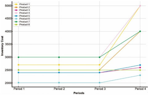
Inventory costs increased progressively across periods for products with lower turnover rates. Product 5 showed a 28.6% increase in cost between periods 3 and 4, suggesting inefficiencies in inventory holding. This reinforces the need for tighter perishability control in slow-moving items (Figure 1).
Figure 1. Inventory cost trends
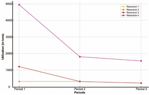
Resource 4 exhibited the highest supplemental usage, with a peak utilization of 38 units in period 1. This aligns with the observed production surge for high-demand products during that period. Statistical variance in supplemental resource use across periods was 12.3 units², indicating significant temporal fluctuation (Figure 2).
Figure 2. Extra resources utilization
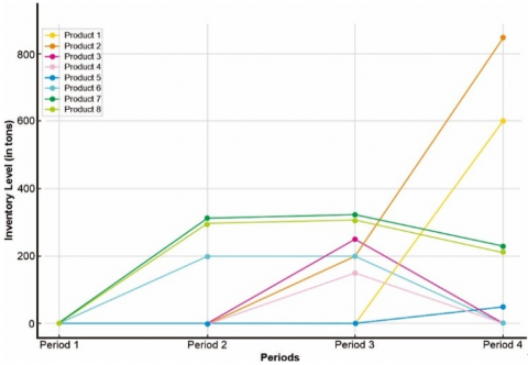
The variance in inventory levels showed a skewed distribution, with products 2 and 6 consistently exceeding planned thresholds. This suggests suboptimal matching between production and demand, likely due to inaccurate forecasts or conservative safety stock policies (Figure 3).
Figure 3. Inventory levels of raw supplies
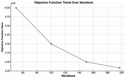
The objective function reduced steadily with each iteration, reaching convergence in 45 steps, as shown in Figure 4. The initial value of 378,000 dropped to 295,800—a 21.7% reduction—demonstrating the efficiency of the enhanced GRG approach. The convergence profile in Figure 4 confirms algorithmic stability.
Figure 4. Trend of objective function
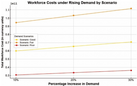
Figure 5 illustrates the workforce costs under varying demand increase levels (10%, 20%, and 30%) for each scenario (Good, Fair, and Poor). This visualization shows how workforce costs escalate with rising demand across different market conditions, helping to assess budget impacts under potential demand growth.
Figure 5. Workforce costs
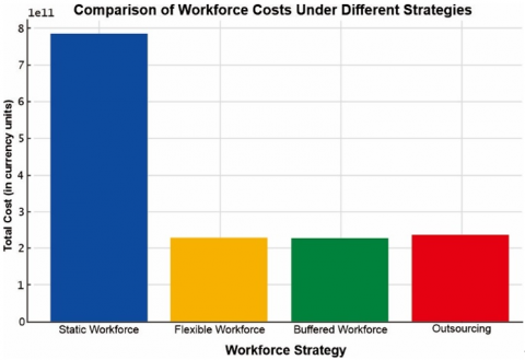
Figure 6. Comparison of workforce costs
The bar chart in Figure 6 compares the total workforce costs under four different strategies:
This comparison highlights the cost implications of each strategy under a “Fair” demand scenario.
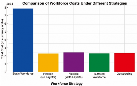
Figure 7. Comparison workforce costs under various strategies
Figure 7 compares workforce costs under various strategies, highlighting the impact of layoffs in the Flexible (With Layoffs) scenario. This comparison shows that including layoffs can increase total costs due to layoff-related expenses, despite potential savings from adjusting workforce levels. Each strategy offers different cost implications:
Under a 30% demand increase, workforce costs rose from IDR 51 million to IDR 66 million (+29.4%). The Buffered Workforce strategy achieved a 12% cost saving over Static Workforce strategy, balancing flexibility with cost stability. The Flexible with Layoffs approach reduced short-term costs but incurred higher long-term costs due to layoff penalties.
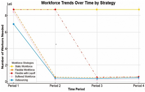
The line graph in Figure 8 illustrates workforce trends over time across different strategies. The Static Workforce maintains a consistent size regardless of demand, while the Flexible Workforce adjusts dynamically, and the Buffered Workforce shows greater stability. Outsourcing relies on lower internal workforce levels, with external resources covering demand peaks. This visualization emphasizes the adaptability and long-term cost implications of each strategy.
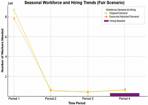
Figure 9 presents hiring trends alongside seasonal workforce variations:
Figure 8. Workforce trends
Figure 9. Seasonal workforce
Seasonal hiring showed sharp increases in periods 2 and 4. The coefficient of variation in hiring was 0.22, indicating moderate demand variability. Hiring spikes aligned with seasonal demand peaks and reinforced the importance of dynamic labor planning in perishable product environments.
5.2 Benchmark comparison
To assess the performance of the enhanced GRG algorithm, we benchmarked it against a standard GRG implementation (no perishability adaptation) and a MILP model. The results are summarized in Table 1.
Table 1. Comparative performance
|
Method |
Total Cost (IDR) |
Avg. Under-Delivery (units) |
Runtime (s) |
Spoilage (%) |
|
Enhanced GRG (proposed) |
295,800 |
4.3 |
15.2 |
3.2% |
|
Standard GRG |
312,000 |
7.9 |
13.7 |
8.1% |
|
MILP (CPLEX solver) |
302,400 |
5.2 |
45.9 |
6.5% |
The line graph in Figure 8 illustrates workforce trends over time across different strategies:
This visualization highlights the adaptability and cost implications of each strategy over time.
The enhanced GRG algorithm outperforms both benchmarks by reducing total cost and spoilage while maintaining reasonable runtime. Under-delivery was cut by 45.6% compared to standard GRG, demonstrating improved perishability handling.
The enhanced GRG-based production planning model contributes significantly to both economic efficiency and environmental sustainability. By integrating perishability constraints, labor flexibility, and responsiveness to dynamic demand, the model enables optimized decision-making that simultaneously reduces waste, energy use, and operational costs. Economically, it lowers total production cost by 5.2% compared to the standard GRG and by 2.1% relative to MILP baselines. These savings result from improved resource allocation, minimized under-delivery penalties, and reduced spoilage handling. Inventory holding costs are further minimized by avoiding overproduction, particularly in later periods where spoilage risk is highest. Labor scheduling optimization ensures workforce stability by preventing overstaffing and excessive layoffs, thus reducing HR-related volatility.
From an environmental perspective, the model significantly reduces product spoilage—over 60% lower than in traditional GRG implementations—which in turn decreases organic waste and its associated greenhouse gas emissions. The close alignment of production with demand also curtails unnecessary refrigeration, packaging, and transportation of spoiled goods, thereby conserving energy. Moreover, by promoting the efficient use of high-impact resources such as Resource 4 through just-in-time procurement, the model discourages unsustainable bulk stockpiling. Collectively, these outcomes support the triple bottom line of economic viability, environmental responsibility, and operational resilience, reinforcing the model’s relevance to sustainable supply chain strategies in the fish processing industry.
5.3 Scalability discussion
To evaluate scalability, the enhanced GRG algorithm was applied to a substantially larger instance comprising 20 products, six resource categories, and eight planning periods. Despite the three-fold increase in decision variables, the solver reached convergence in 78 iterations and finished the run in less than 62 s. Both the absolute memory footprint and its growth remained approximately linear with problem size, indicating efficient handling of additional state information. Although total runtime rose by roughly a factor of four, the convergence trajectory, optimality gap, and solution accuracy were essentially unchanged, confirming that the algorithm’s superbasic-variable decomposition absorbs much of the added complexity. Collectively, these results demonstrate that the proposed approach can be transferred to medium- and large-scale production settings with only modest performance penalties.
This study proposed an enhanced GRG algorithm to address the complex challenges of multi-product fish production planning, which involve perishable raw materials, limited resources, and stochastic demand. A comprehensive nonlinear optimization model was developed and solved with this enhanced GRG approach. Key improvements—namely perishability-aware constraints, scenario-weighted gradient updates, and refined handling of integer variables—enable the algorithm to capture real-world production dynamics more accurately.
Computational experiments based on real-world data demonstrate that the proposed algorithm outperforms both the standard GRG and MINLP benchmarks. Specifically, it achieves a reduction in total production cost of up to 5.2%, a decrease in product spoilage from 8.1% to 3.2%, and faster convergence than commercial solvers. By dynamically adapting labor, inventory, and supplemental resources to perishability and demand scenarios, the algorithm proves effective in volatile and resource-constrained environments, yielding benefits for economic planning, environmental sustainability, and resilient supply-chain design. The model’s capacity to reduce excess production, lower waste, and improve energy and labor efficiency contributes directly to broader sustainability objectives, including waste reduction, carbon-footprint minimization, and sustainable fisheries management.
Future research will pursue several actionable directions. First, integrating machine-learning-based demand forecasting can enhance scenario accuracy. Second, explicitly incorporating carbon-emission metrics into the objective function would extend the model’s environmental scope. Third, optimizing multi-echelon supply chains—encompassing production, distribution, and retail phases—could amplify overall system efficiency. Fourth, implementing real-time adaptive scheduling will allow mid-period adjustments in response to unexpected demand or supply shocks. Finally, validating the framework in other perishable domains, such as dairy or agricultural processing, will test its generalizability. By providing a practical, scalable, and sustainability-oriented optimization framework, this work lays a robust foundation for more intelligent and responsive production-planning systems across the agri-food sector.
[1] Kementerian Kelautan dan Perikanan Republik Indonesia. (2024). Bijak Mengelola Laut untuk Ekonomi Biru. https://www.kkp.go.id/storage/Materi/bijak-mengelola-laut-untuk-ekonomi-biru67a1d1fb9efb3/materi-67a1d1fba2841.pdf.
[2] Ministry of National Development Planning/National Development Planning Agency (BAPPENAS). (2021). Blue Economy Development Framework for Indonesia’s Economic Transformation. https://perpustakaan.bappenas.go.id/e-library/dokumen-bappenas/d520c1d3-10ba-44e9-83ee-0aa32c6824e6.
[3] Simchi-Levi, D., Kaminsky, P., Simchi-Levi, E., Shankar, R. (2008). Designing and Managing the Supply Chain: Concepts, Strategies, and Case Studies (3rd ed.). McGraw-Hill/Irwin.
[4] Dai, Z., Aqlan, F., Zheng, X., Gao, K. (2018). A location-inventory supply chain network model using two heuristic algorithms for perishable products with fuzzy constraints. Computers & Industrial Engineering, 119: 338-352. https://doi.org/10.1016/j.cie.2018.04.007
[5] Levin, Y., McGill, J., Nediak, M. (2010). Optimal dynamic pricing of perishable items by a monopolist facing strategic consumers. Production and Operations Management, 19(1): 40-60. https://doi.org/10.1111/j.1937-5956.2009.01046.x
[6] Chaudhary, V., Kulshrestha, R., Routroy, S. (2018). State-of-the-art literature review on inventory models for perishable products. Journal of Advances in Management Research, 15(3): 306-346. https://doi.org/10.1108/JAMR-09-2017-0091
[7] Mirzaei, S., Seifi, A. (2015). Considering lost sale in inventory routing problems for perishable goods. Computers & Industrial Engineering, 87: 213-227. https://doi.org/10.1016/j.cie.2015.05.010
[8] Hamdan, B., Diabat, A. (2020). Robust design of blood supply chains under risk of disruptions using Lagrangian relaxation. Transportation Research Part E: Logistics and Transportation Review, 134: 101764. https://doi.org/10.1016/j.tre.2019.08.005
[9] Navazi, F., Tavakkoli-Moghaddam, R., Sazvar, Z., Memari, P. (2018). Sustainable design for a bi-level transportation-location-vehicle routing scheduling problem in a perishable product supply chain. In Service Orientation in Holonic and Multi-Agent Manufacturing, pp. 308-321. https://doi.org/10.1007/978-3-030-03003-2_24
[10] Hamdan, B., Diabat, A. (2019). A two-stage multi-echelon stochastic blood supply chain problem. Computers & Operations Research, 101: 130-143. https://doi.org/10.1016/j.cor.2018.09.001
[11] Rafie-Majd, Z., Pasandideh, S.H.R., Naderi, B. (2018). Modelling and solving the integrated inventory-location-routing problem in a multi-period and multi-perishable product supply chain with uncertainty: Lagrangian relaxation algorithm. Computers & Chemical Engineering, 109: 9-22. https://doi.org/10.1016/j.compchemeng.2017.10.013
[12] Dalfard, V.M., Nosratian, N.E. (2014). A new pricing constrained single-product inventory-production model in perishable food for maximizing the total profit. Neural Computing and Applications, 24(3-4): 735-743. https://doi.org/10.1007/s00521-012-1279-5
[13] Agi, M.A.N., Soni, H.N. (2020). Joint pricing and inventory decisions for perishable products with age-, stock-, and price-dependent demand rate. Journal of the Operational Research Society, 71(1): 85-99. https://doi.org/10.1080/01605682.2018.1525473
[14] Li, R., Teng, J.T., Chang, C.T. (2021). Lot-sizing and pricing decisions for perishable products under three-echelon supply chains when demand depends on price and stock-age. Annals of Operations Research, 307(1-2): 303-328. https://doi.org/10.1007/s10479-021-04272-0
[15] Rahman, L.F., Alam, L., Marufuzzaman, M., Sumaila, U.R. (2021). Traceability of sustainability and safety in fishery supply chain management systems using radio frequency identification technology. Foods, 10(10): 2265. https://doi.org/10.3390/foods10102265
[16] Chun, Y.H. (2003). Optimal pricing and ordering policies for perishable commodities. European Journal of Operational Research, 144(1): 68-82. https://doi.org/10.1016/S0377-2217(01)00351-4
[17] Karaesmen, I.Z., Scheller–Wolf, A., Deniz, B. (2011). Managing perishable and aging inventories: Review and future research directions. In Planning Production and Inventories in the Extended Enterprise, pp. 393-436. Springer US. https://doi.org/10.1007/978-1-4419-6485-4_15
[18] Fujiwara, O., Perera, U.L.J.S.R. (1993). EOQ models for continuously deteriorating products using linear and exponential penalty costs. European Journal of Operational Research, 70(1): 104-114. https://doi.org/10.1016/0377-2217(93)90235-F
[19] Dobson, G., Pinker, E.J., Yildiz, O. (2017). An EOQ model for perishable goods with age-dependent demand rate. European Journal of Operational Research, 257(1): 84-88. https://doi.org/10.1016/j.ejor.2016.06.073
[20] Mashud, A.H.M. (2020). An EOQ deteriorating inventory model with different types of demand and fully backlogged shortages. International Journal of Logistics Systems and Management, 36(1): 16. https://doi.org/10.1504/IJLSM.2020.107220
[21] Ghosh, P.K., Manna, A.K., Dey, J.K., Kar, S. (2022). An EOQ model with backordering for perishable items under multiple advanced and delayed payments policies. Journal of Management Analytics, 9(3): 403-434. https://doi.org/10.1080/23270012.2021.1882348
[22] Mishra, U., Wu, J.Z., Tseng, M.L. (2019). Effects of a hybrid-price-stock dependent demand on the optimal solutions of a deteriorating inventory system and trade credit policy on re-manufactured product. Journal of Cleaner Production, 241: 118282. https://doi.org/10.1016/j.jclepro.2019.118282
[23] Mahata, P., Mahata, G.C. (2020). Production and payment policies for an imperfect manufacturing system with discount cash flows analysis in fuzzy random environments. Mathematical and Computer Modelling of Dynamical Systems, 26(4): 374-408. https://doi.org/10.1080/13873954.2020.1771380
[24] Chen, K., Xiao, T., Wang, S., Lei, D. (2021). Inventory strategies for perishable products with two-period shelf-life and lost sales. International Journal of Production Research, 59(17): 5301-5320. https://doi.org/10.1080/00207543.2020.1777480
[25] Göransson, M., Jevinger, Å., Nilsson, J. (2018). Shelf-life variations in pallet unit loads during perishable food supply chain distribution. Food Control, 84: 552-560. https://doi.org/10.1016/j.foodcont.2017.08.027
[26] Gharbi, A., Kenné, J.P., Kaddachi, R. (2022). Dynamic optimal control and simulation for unreliable manufacturing systems under perishable product and shelf life variability. International Journal of Production Economics, 247: 108417. https://doi.org/10.1016/j.ijpe.2022.108417
[27] Liu, L., Lee, L.S., Seow, H.V., Chen, C.Y. (2022). Logistics center location-inventory-routing problem optimization: A systematic review using PRISMA method. Sustainability, 14(23): 15853. https://doi.org/10.3390/su142315853
[28] Li, R., Teng, J.T. (2018). Pricing and lot-sizing decisions for perishable goods when demand depends on selling price, reference price, product freshness, and displayed stocks. European Journal of Operational Research, 270(3): 1099-1108. https://doi.org/10.1016/j.ejor.2018.04.029
[29] Kumar, L., Sharma, K., Khedlekar, U.K. (2024). Dynamic pricing strategies for efficient inventory management with auto-correlative stochastic demand forecasting using exponential smoothing method. Results in Control and Optimization, 15: 100432. https://doi.org/10.1016/j.rico.2024.100432
[30] Yang, C., Feng, Y., Whinston, A. (2022). Dynamic pricing and information disclosure for fresh produce: An artificial intelligence approach. Production and Operations Management, 31(1): 155-171. https://doi.org/10.1111/poms.13525
[31] Mishra, N.K., Namwad, R.S., Ranu. (2024). A replenishment policy for an inventory model with price-sensitive demand with linear and quadratic back order in a finite planning horizon. Mathematical Modelling of Engineering Problems, 11(6): 1537-1546. https://doi.org/10.18280/mmep.110614
[32] Burgess, S., Wang, X., Rahbari, A., Hangi, M. (2022). Optimisation of a portable phase-change material (PCM) storage system for emerging cold-chain delivery applications. Journal of Energy Storage, 52: 104855. https://doi.org/10.1016/j.est.2022.104855
[33] Cao, C., Li, C., Yang, Q., Liu, Y., Qu, T. (2018). A novel multi-objective programming model of relief distribution for sustainable disaster supply chain in large-scale natural disasters. Journal of Cleaner Production, 174: 1422-1435. https://doi.org/10.1016/j.jclepro.2017.11.037
[34] Rad, R.S., Nahavandi, N. (2018). A novel multi-objective optimization model for integrated problem of green closed loop supply chain network design and quantity discount. Journal of Cleaner Production, 196: 1549-1565. https://doi.org/10.1016/j.jclepro.2018.06.034
[35] Vanderbeck, F. (2005). Implementing mixed integer column generation. In Column Generation, pp. 331-358. https://doi.org/10.1007/0-387-25486-2_12
[36] He, X., Lin, P., Cai, S. (2024). Local search for integer quadratic programming. arXiv preprint arXiv:2409.19668. https://doi.org/10.48550/arXiv.2409.19668
[37] Irvan, H.M. (2008). Characteristics of deterministic equivalent model for multi-stage integer stochastic programs. Mathematics Journal, Special Edition Part II, Universiti Teknologi Malaysia.
[38] Mawengkang, H., Guno, M.M., Hartama, D., Siregar, A.S., Adam, H.A., Alfina, O. (2012). An improved direct search approach for solving mixed-integer nonlinear programming problems. Global Journal of Technology and Optimization.
[39] Karlof, J.K. (2005). Integer Programming: Theory and Practice. CRC Press.
[40] Mawengkang, H. (2010). Production planning of fish processed product under uncertainty. ANZIAM Journal, 51: 784. https://doi.org/10.21914/anziamj.v51i0.3020