Diah Safitri![]() | Gunardi*
| Gunardi*![]() | Nanang Susyanto
| Nanang Susyanto![]() | Winita Sulandari
| Winita Sulandari![]()
© 2025 The authors. This article is published by IIETA and is licensed under the CC BY 4.0 license (http://creativecommons.org/licenses/by/4.0/).
OPEN ACCESS
The assumption of homoscedastic errors is fundamental in many time series models, but financial data often exhibit heteroscedasticity. This study focuses on the development of Singular Spectrum Analysis (SSA)-based time series modeling with heteroscedasticity. The proposed model, termed Singular Spectrum Analysis–Autoregressive Integrated Moving Average–Generalized Autoregressive Conditional Heteroscedasticity (SSA-ARIMA-GARCH), uses SSA to decompose the time series into signal and noise. The modeling focuses on signals because they contribute significantly to the overall structure of the time series. Two algorithms are discussed in this study. The first algorithm is to model the signal with ARIMA and ignore the noise by assuming that the model built from the signal will better represent the actual data because it has been free from noise. The second algorithm is to model the signal and noise separately, each using a distinct ARIMA model. The two models are then applied to simulations and the daily stock price data of PT Astra International Tbk (ASII). Each model is evaluated based on mean absolute error (MAE), and the results are then compared with those obtained by ARIMA as the benchmark model. To demonstrate that the proposed SSA-ARIMA-GARCH can reduce the effects of heteroscedasticity in the data, we observed the p-value obtained by the Ljung-Box test. The larger the p-value, the smaller the heteroscedasticity effect. The experimental results showed that the proposed SSA-ARIMA-GARCH produced a p-value that was 39 percent larger than that of ARIMA-GARCH, and it reduced the MAE by nearly 34 percent.
heteroscedasticity, hybrid models, Singular Spectrum Analysis (SSA), Autoregressive Integrated Moving Average (ARIMA), Generalized Autoregressive Conditional Heteroscedasticity (GARCH), time series forecasting, stock price prediction
A time series is an ordered sequence of observations, and there has been a lot of activity in the field of time series analysis in recent years. The general assumption in time series modeling is that the variance of errors is constant. Unfortunately, this does not always occur with financial data. Generally, financial data is dynamic with high volatility or heteroscedasticity, so mean and variance forecasting is required to obtain accurate forecasts. The commonly used model is Autoregressive Integrated Moving Average-ARIMA-Generalized Autoregressive Conditional Heteroscedasticity (ARIMA-GARCH) to deal with heteroscedasticity, with the ARIMA as the mean model and GARCH as the variance model. Box and Jenkins introduced the ARIMA method in 1970. The GARCH model is an expansion of the Autoregressive Conditional Heteroscedasticity (ARCH). The ARCH introduced by Engle [1] and Bollerslev [2] first proposed the GARCH model. GARCH theory was described by Enders [3] and Paolella [4]. According to the research [3], ARCH is the model that uses conditional variance as an autoregressive process using squares of the estimated residuals, whereas the generalized ARCH (GARCH) allows for both autoregressive and moving average components in the heteroscedastic variance.
Abreu et al. [5] applied ARIMA-GARCH and Singular Spectrum Analysis (SSA) methods to model minute-level EUR/USD exchange rate data. They evaluated the models across three distinct market conditions—upward trend, downward trend, and neutral or undefined trend—using closing ask prices. In their study, SSA was employed as a standalone method, not in a hybridized form. According to Hassani and Thomakos [6], SSA is a relatively recent yet effective tool in time series analysis, having found applications across diverse fields [7-10]. Elsner [11] notes that SSA primarily aims to break down a time series into multiple reconstructed components. As explained by Golyandina and Zhigljavsky [12], the technique relies on the singular value decomposition (SVD) of a trajectory matrix derived from the original series. Since SSA does not assume an underlying statistical model, it offers a high degree of flexibility in its applications. The foundational theory of SSA is elaborated in several key references, including Golyandina and Zhigljavsky [12], Degiannakis et al. [13], Golyandina et al. [14], Hassani [15], and Golyandina and Korobeynikov [16].
SSA has been effectively applied to analyze complex datasets. For instance, Sulandari et al. [17-19] integrated SSA with neural networks (NN) to deal with time series data containing nonlinear patterns. Meanwhile, Suhartono et al. [20] introduced a hybrid method called SSA–TSR–ARIMA, which is aimed at forecasting time series with both trend and seasonal characteristics. In this method, SSA breaks down the original series into core components: trend, seasonality, and noise. The trend and calendar effects are then modeled using Time Series Regression (TSR), while the seasonal and noise parts are handled by ARIMA. Irmawati et al. [21] developed a combined SSA–ARIMA approach to enhance prediction accuracy of the Farmer’s Terms of Trade (FTT) in East Java. Their model involves two steps: first, SSA is used to separate the series into signal (trend and seasonality) and noise, then ARIMA is applied to model the residuals. Arteche and Garcia-Enriquez [22] applied SSA in estimating Value at Risk within Stochastic Volatility Models.
This study discusses the use of the SSA–ARIMA model for time series data with heteroscedasticity, and the GARCH model is applied to model the variance of the residuals from the SSA–ARIMA approach, a step that is not addressed in the works of Suhartono et al. [20] and Irmawati et al. [21]. Meanwhile, variance modeling for heteroscedasticity is very important for financial data, so a modification of the hybrid model is necessary.
The decomposition into signal and noise aims to identify the part of the data that carries important information (signal) more easily. Signals contribute significantly to the data, while noise makes a small contribution. SSA is a decomposition method that can decompose data into signal and noise. Therefore, this paper proposes a hybrid SSA-ARIMA-GARCH model to overcome time series with heteroscedasticity effects. In the hybrid SSA-ARIMA-GARCH model, SSA-ARIMA is the mean model, and GARCH is the variance model. We decompose the time series using SSA into signal and noise and construct a model that better represents the signal.
The novelty of this study lies in the application of SSA as an approach to address the issue of heteroscedasticity in time series data. In this study, SSA is used to decompose the time series into two main components: signal and noise. After the decomposition process, the next step is modeling using the ARIMA approach, which is applied in two different treatments. In the first treatment, the ARIMA model is built only on the signal component, while the noise component is ignored. In the second treatment, ARIMA is applied to both the signal and noise components. This second treatment is performed when there is autocorrelation in the noise component. Furthermore, if the residuals from the ARIMA model still exhibit ARCH effects, they are further modeled using the GARCH model to accommodate the heteroscedasticity. This approach is referred to as the hybrid SSA–ARIMA–GARCH model.
2.1 Singular spectrum analysis
The SSA algorithm involves four main steps: embedding, singular value decomposition, grouping, and diagonal averaging. Details of this algorithm are explained in Golyandina and Zhigljavsky [12], Golyandina et al. [14], and Hassani [15]. The steps are outlined as follows: Let $X=X_N= \left(x_1, \ldots, x_N\right)$ be a real-valued time series of length $N$. Assume that $N>2$ and $X$ is not a zero series. The window length is represented by $L$, where $L \leq N / 2$, and $N$ is the total number of data points in the time series.
In the embedding step, the original time series is transformed into a set of lagged vectors, each of which is multidimensional. This process creates $K=N-L+1$ lagged vectors:
$X_i=\left(x_i, \ldots, x_{i+L-1}\right)^T,(1 \leq i \leq K)$ (1)
where, each vector has a dimension of $L$. These vectors are used to construct the $L$-trajectory matrix of the time series $X$, defined as:
$\mathbf{X}=\left(x_{i j}\right)_{i, j=1}^{L, K}=\left[\begin{array}{ccccc}x_1 & x_2 & x_3 & \ldots & x_K \\ x_2 & x_3 & x_4 & \ldots & x_{K+1} \\ x_3 & x_4 & x_5 & \ldots & x_{K+2} \\ \vdots & \vdots & \vdots & \ddots & \vdots \\ x_L & x_{L+1} & x_{L+2} & \ldots & x_N\end{array}\right]$
Here, the lagged vectors $X_i$ are the columns of the matrix $\mathbf{X}$. Both the rows and columns represent subseries of the original series. This matrix $\mathbf{X}$ is a type of Hankel matrix, as explained further by Hassani et al. [23].
The second step is to perform Singular Value Decomposition (SVD) on the trajectory matrix $\mathbf{X}$. Let $\mathbf{S}= \mathbf{X X}^{\mathbf{T}}$, and let $\lambda_1, \lambda_2, \ldots, \lambda_{\mathrm{L}}$ be the eigenvalues of $\mathbf{S}$ arranged in decreasing order ($\lambda_1 \geq \cdots \geq \lambda_{\mathrm{L}} \geq 0$). The corresponding eigenvectors of $\mathbf{S}$ are denoted as $U_1, \ldots, U_L$, forming an orthonormal set. Define $d$ as the rank of $\mathbf{S}$, that is, $d=$ rank $\mathbf{X}=\max \left\{\mathrm{i}\right.$, such that $\left.\lambda_{\mathrm{i}}>0\right\}$. Then, for each $i=1, \ldots, d$, define $V_i=\mathbf{X}^T U_i / \sqrt{\lambda_{\mathrm{i}}}(i=1, \ldots, d)$. Using these values, the SVD of matrix $\mathbf{X}$ can be expressed as:
$\mathbf{X}=\mathbf{X}_1+\mathbf{X}_2+\cdots+\mathbf{X}_d$ (2)
where, each component $\mathbf{X}_{\mathbf{i}}=\sqrt{\lambda_{\mathrm{i}}} U_i V_i^T$. The set $\left(\sqrt{\lambda_{\mathrm{i}}}, U_i, V_i\right)$ is known as the $i$-th eigen triple of the SVD. Golyandina et al. [14] considered the decomposition in Eq. (2). Two time series $F_1$ and $F_2$ are said to be separable if there is a subset of indices $I \subset\{1, \ldots, d\}$ such that $\mathbf{X}_1=\sum_{i \in I} \mathbf{X}_i$ and $\mathbf{X}_2=\sum_{i \in I} \mathbf{X}_i$. When such separation is possible, the proportion of contribution explained by $\mathbf{X}_1$ can be measured using the ratio of eigen values:
$\sum_{i \in I} \lambda_i / \sum_{i=1}^L \lambda_i$ (3)
In the grouping step, the index set $\{1, \ldots, d\}$ is divided into $m$ separate, non-overlapping subsets: $I_1, \ldots, I_m$. Based on Eq. (2), this results in the following decomposition:
$\mathbf{X}=\mathbf{X}_{\mathrm{I}_1}+\cdots+\mathbf{X}_{\mathrm{I}_m}$ (4)
This selection of the index subsets $\boldsymbol{I}_1, \ldots, \boldsymbol{I}_m$ is referred to as eigen triple grouping.
$y_k=\left\{\begin{array}{c}\frac{1}{k} \sum_{m=1}^k y_{m, k-m+1}^* \text { for } 1 \leq k<L^* \\ \frac{1}{L^*} \sum_{m=1}^{L^*} y_{m, k-m+1}^* \text { for } L^* \leq k<K^* \\ \frac{1}{N-k+1} \sum_{m=k-K^*+1}^{N-K^*+1} y_{m, k-m+1}^* \text { for } K^*<k \leq N\end{array}\right.$ (5)
The final step is to convert each matrix from the group decomposition in Eq. (4) into a time series of length $N$. Let $\mathbf{Y}$ be an $L \times K$ matrix with elements $y_{i j}$, where $1 \leq i \leq L, 1 \leq j \leq K$, and let $N=L+K-1$. Define $y_{i j}^*=y_{i j}$ when $L<K$, and $y_{i j}^*=y_{j i}$ otherwise. This matrix $\mathbf{Y}$ is then transformed into a time series $y_1, \ldots, y_N$ using the above equations.
Applying this diagonal averaging process Eq. (5) to each matrix results in a reconstructed time series $\tilde{X}^k= \left(\tilde{x}_1^{(k)}, \ldots, \tilde{x}_N^{(k)}\right)$. As a result, the original series $x_1, \ldots, x_N$ can be represented as the sum of $m$ reconstructed components:
$x_n=\sum_{k=1}^m \tilde{x}_n^{(k)}(n=1,2, \ldots, N)$ (6)
2.2 ARIMA-GARCH hybrid model
The general ARIMA (p,d,q) model can be found by Wei [24], Brockwell and Davis [25] as follows:
$\phi_p B(1-B)^d X_t=\theta_0+\theta_q(B) a_t$ (7)
where,
$\phi_p(B)=1-\phi_1 B-\cdots-\phi_p B^p$ (8)
and
$\theta_q(B)=1-\theta_1 B-\cdots-\theta_q B^q$ (9)
$\phi$ is a parameter of the autoregressive model, $\theta$ is the parameter of the moving average, $p$ and $q$ are used to indicate the autoregressive and moving average orders, respectively. In the study conducted by Tsay [26], the basic idea of ARCH models is that the residuals of the mean equation $\left(a_t\right)$ are serially uncorrelated, but dependent, and the dependence of $a_t$ can be described by a quadratic function of its lagged values. An $\operatorname{ARCH}(p)$ model assumes that:
$a_t=\sigma_t v_t$ (10)
$\sigma_t^2=\alpha_0+\alpha_1 a_{t-1}^2+\cdots+\alpha_p a_{t-p}^2$ (11)
where, $\left\{v_t\right\}$ is a sequence of independent and identically distributed (iid) random variables with mean 0 and variance 1. The ARCH model was introduced by Engle [1], and then the GARCH model is an expansion of the ARCH model and was introduced by Bollerslev [2]. Tsay [26] let $a_t$ the residuals of the mean equation, $a_t$ uncorrelated and follow a GARCH (p , q) model if:
$a_t=\sigma_t v_t$ (12)
$\sigma_t^2=\alpha_0+\sum_{i=1}^p \alpha_i a_{t-i}^2+\sum_{j=1}^q \beta_j \sigma_{t-j}^2$ (13)
where, $\left\{v_t\right\}$ is a sequence of iid random variables with mean 0 and variance 1. The explanation of the GARCH model can be found by Francq and Zakoïan [27], Paolella [4], and Neusser [28].
A hybrid SSA-ARIMA-GARCH model, with SSA-ARIMA serving as the mean model and GARCH serving as the variance model, is the goal of this research. We use SSA to decompose time series into signal and noise.
3.1 The proposed algorithm
(1). Decomposing ARIMA-GARCH generated series using SSA.
$Z_t=Z_t^{(1)}+Z_t^{(2)}$ (14)
where,
$Z_t=$ ARIMA-GARCH generated series,
$Z_t^{(1)}=$ the signal of the ARIMA-GARCH generated series, and
$Z_t^{(2)}=$ the noise of the ARIMA-GARCH generated series.
(2). There are two treatments.
(3). Evaluating the forecasting accuracy. This work considers MAE as the forecasting accuracy value.
(4). Examining residuals for heteroscedasticity effects based on autocorrelation of quadratic residuals, with the statistic.
$Q=T(T+2) \sum_{h=1}^N \frac{\hat{\rho}_{X^2}^2(h)}{T-h}$ (15)
$\hat{\rho}_{X^2}(h)=\frac{\sum_{t=h+1}^T\left(\hat{X}_t^2-\hat{\sigma}^2\right)\left(\hat{X}_{t-h}^2-\hat{\sigma}^2\right)}{\sum_{t=1}^T\left(\hat{X}_t^2-\hat{\sigma}^2\right)^2}$ (16)
and
$\hat{\sigma}^2=\frac{1}{T} \sum_{t=1}^T \hat{X}_t^2$ (17)
where,
$T=$ sample size,
$X_t=$ residuals,
$\sigma^2=$ variance,
$\rho_z=$ correlation function of process $\left\{Z_t\right\}$.
(5). Constructing a GARCH model (13) if the residuals have heteroscedasticity effects.
Checking for residuals heteroscedasticity effects remaining after estimating the GARCH model using Eq. (16), if none remain, it suggests that the GARCH model is suitable for describing the series volatility.
(6). Interpreting the obtained SSA-ARIMA-GARCH model.
This study introduces a hybrid SSA-ARIMA approach as the underlying forecasting model, where SSA is first employed to separate the time series into its signal and noise components. Forecast performance is evaluated using the Mean Absolute Error (MAE) metric.
$\operatorname{MAE}=\frac{1}{n} \sum_{i=1}^n\left|Z_t-\hat{Z}_t\right|$ (18)
where,
$Z_t=$ actual data for period t,
$\hat{Z}_t=$ prediction for period t,
$n=$ the number of periods.
3.2 Proposition
Let $Z_t$ be a time series with $t=1, \ldots, n . Z_t$ is decomposed using SSA into:
$Z_t=Z_t^{(1)}+Z_t^{(2)}$ (19)
where, $Z_t^{(1)}$ as the signal and $Z_t^{(2)}$ as the noise, assuming that there is autocorrelation in the noise.
Considered in two treatments:
i. First treatment: $\hat{Z}_t=\hat{Z}_t^{(1)}$
ii. Second treatment: $\hat{Z}_t=\hat{Z}_t^{(1)}+\hat{Z}_t^{(2)}$
where, $\hat{Z}_t^{(1)}$ as the forecast from the signal and $\hat{Z}_t^{(2)}$ as the forecast from the noise. If the MAE from first treatment $\left(\mathrm{MAE}_{\mathrm{I}}\right):$
$\mathrm{MAE}_{\mathrm{I}}=\frac{1}{n} \sum_{t=1}^n\left|Z_t-\hat{Z}_{t(I)}\right|$ (20)
and MAE second treatment $\left(\mathrm{MAE}_{\mathrm{II}}\right)$
$\mathrm{MAE}_{\mathrm{II}}=\frac{1}{n} \sum_{t=1}^n\left|Z_t-\hat{Z}_{t(I I)}\right|$ (21)
then
$\mathrm{MAE}_{\mathrm{I}} \geq \mathrm{MAE}_{\mathrm{II}}$ (22)
Proof:
$\mathrm{MAE}_{\mathrm{II}}=\frac{1}{n} \sum_{t=1}^n\left|Z_t-\hat{Z}_{t(I I)}\right|$ (23)
$\mathrm{MAE}_{\mathrm{II}}=\frac{1}{n} \sum_{t=1}^n\left|\left(Z_t^{(1)}-\hat{Z}_t^{(1)}\right)+\left(Z_t^{(2)}-\hat{Z}_t^{(2)}\right)\right|$ (24)
$\mathrm{MAE}_{\mathrm{II}}=\frac{1}{n} \sum_{t=1}^n\left|Z_t^{(1)}-\hat{Z}_t^{(1)}+Z_t^{(2)}-\hat{Z}_t^{(2)}\right|$ (25)
$\mathrm{MAE}_{\mathrm{I}}=\frac{1}{n} \sum_{t=1}^n\left|Z_t-\hat{Z}_{t(I)}\right|$ (26)
$\mathrm{MAE}_{\mathrm{I}}=\frac{1}{n} \sum_{t=1}^n\left|Z_t^{(1)}-\hat{Z}_t^{(1)}+Z_t^{(2)}\right|$ (27)
$\mathrm{MAE}_{\mathrm{I}}=\frac{1}{n} \sum_{t=1}^n\left|Z_t^{(1)}-\hat{Z}_t^{(1)}+Z_t^{(2)}+\hat{Z}_t^{(2)}-\hat{Z}_t^{(2)}\right|$ (28)
$\mathrm{MAE}_{\mathrm{I}}=\frac{1}{n} \sum_{t=1}^n\left|\left(Z_t^{(1)}-\hat{Z}_t^{(1)}+Z_t^{(2)}-\hat{Z}_t^{(2)}\right)+\left(\hat{Z}_t^{(2)}\right)\right|$ (29)
$\mathrm{MAE}_{\mathrm{I}}=\frac{1}{n} \sum_{t=1}^n\left|\left(Z_t^{(1)}-\hat{Z}_t^{(1)}+Z_t^{(2)}-\hat{Z}_t^{(2)}\right)-\left(-\hat{Z}_t^{(2)}\right)\right|$ (30)
$\operatorname{MAE}_{\mathrm{I}} \geq \frac{1}{n} \sum_{t=1}^n\left|\left(Z_t^{(1)}-\hat{Z}_t^{(1)}+Z_t^{(2)}-\hat{Z}_t^{(2)}\right)\right|-\frac{1}{n} \sum_{t=1}^n\left|\hat{Z}_t^{(2)}\right|$ (31)
$\mathrm{MAE}_{\mathrm{I}} \geq \mathrm{MAE}_{\mathrm{II}}-\frac{1}{n} \sum_{i=1}^n\left|\hat{Z}_t^{(2)}\right|$ (32)
Since component $\frac{1}{n} \sum_{i=1}^n\left|\hat{Z}_t^{(2)}\right|$ always has a positive value, and according to Golyandina et al. [14], noise has a small contribution value (3), then it is proven that:
$M A E_I \geq M A E_{I I}$ (33)
The steps conducted in the experimental results are as follows: decomposition is performed using SSA with a window length parameter $L \leq N / 2$, followed by ARIMA modeling. The optimal ARIMA order is determined by selecting the model that produces the smallest MAE. The residuals of the resulting SSA–ARIMA model are then examined using the Ljung–Box test on the squared residuals and the ARCH–Lagrange Multiplier (LM) test to detect the presence of any remaining ARCH effects. If ARCH effects are detected, a GARCH model is applied to the residuals of the SSA–ARIMA model. The best GARCH model is selected based on the lowest AIC value, and its adequacy is confirmed by ensuring that the residuals no longer exhibit ARCH effects, as indicated by the results of the Ljung–Box and ARCH–LM tests.
4.1 Simulated data
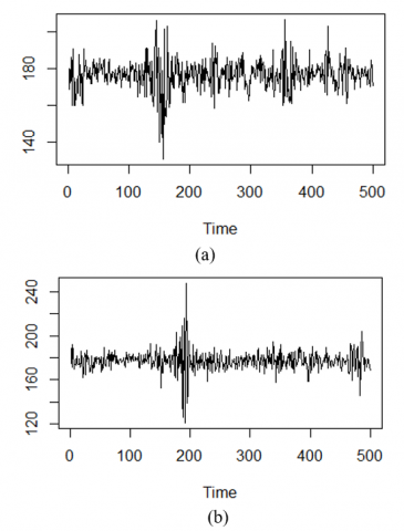
In this research, the simulation study uses the four ARIMA-GARCH models with ARIMA (7) as the mean model and GARCH (13) as the variance model. The simulation data were generated using R software with the time series plot can be seen in Figure 1.
Figure 1. Time series plot of simulated data
(a) ARIMA(1,0,1)-GARCH(2,1) model with parameter
$\left[\phi_1, \theta_1, \alpha_0, \alpha_1, \alpha_2, \beta_1\right]=[0.8,0.18,5,0.21,0.1407,0.6]$
(b) ARIMA(1,0,1)-GARCH(3,1) model with parameter
$\left[\phi_1, \theta_1, \alpha_0, \alpha_1, \alpha_2, \alpha_3, \beta_1\right]=[0.8,0.18,5,0.123,0.28899$, 0.198, 0.39]
(c) ARIMA(2,0,2)-GARCH(2,1) model with parameter
$\left[\phi_1, \phi_2, \theta_1, \theta_2, \alpha_0, \alpha_1, \alpha_2, \beta_1\right]=$$[0.8897,-0.4858,-0.2279,0.2488,5,0.21,0.1407,0.6]$
(d) ARIMA(2,0,)-GARCH(3,1) model with parameter
$\left[\phi_1, \phi_2, \theta_1, \theta_2, \alpha_0, \alpha_1, \alpha_2, \alpha_3, \beta_1\right]=$[0.8897, -0.4858, -0.2279, 0.2488, 5, 0.123, 0.28899, 0.198, 0.39]
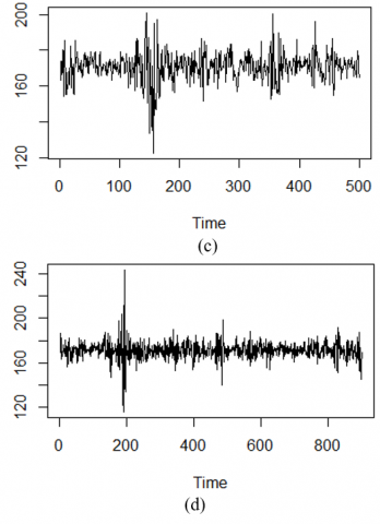
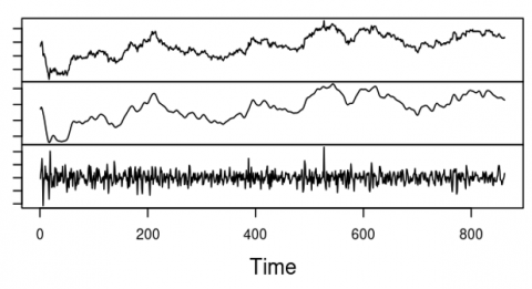
The SSA model was constructed on each series generated, with window length $L(L \leq N / 2)$. The series of ARIMA ( $2,0,2$ )-GARCH( 3,1 ) model can be decomposed into two component groups: the first component is signal, and the second component is noise. Components from decomposition SSA depicted in Figure 2.
Figure 2. Components resulting from decomposition SSA
Table 1. MAE value for the generated series
|
Model of the Generated Series |
MAE |
||
|
ARIMA |
SSA-ARIMA (I) |
SSA-ARIMA (II) |
|
|
ARIMA(1,0,1)-GARCH(2,1) |
6.01 |
5.58 |
5.52 |
|
ARIMA(1,0,1)-GARCH(3,1) |
6.00 |
5.12 |
5.06 |
|
ARIMA(2,0,2)-GARCH(2,1) |
5.97 |
5.28 |
5.21 |
|
ARIMA(2,0,2)-GARCH(3,1) |
5.41 |
4.71 |
4.62 |
In this paper, we conducted both ARIMA modeling without SSA decomposition and SSA-ARIMA modeling, which applies ARIMA after SSA decomposes the data. Decomposition of the time series was performed using SSA to separate the signal and noise, followed by ARIMA modeling on the signal. Based on the residual independence check, the noise still contained correlation, so ARIMA modeling was performed on the noise. Forecasting is the sum of forecasting on signal and noise.
In the fourth set of generated data, it can be seen in Table 1 that the SSA-ARIMA has smaller MAE value than ARIMA, which can be interpreted as the model having the highest forecasting accuracy. The independence of the residuals did not contain a correlation. Afterward, the heteroscedasticity effect was investigated using the squared residuals test for serial correlation. The residuals displayed heteroscedasticity, and a GARCH model will explain the dynamic nature of the standard deviations. In the fourth generated data set, the GARCH model order decreases, initially from order (2,1) and (3,1) to order (1,1).
4.2 Real data
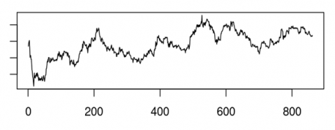
Since the simulation study shows that SSA-ARIMA-GARCH raises the accuracy value of the mean model prediction in time series data and reduces the order of the GARCH model, we apply SSA-ARIMA-GARCH to heteroscedastic real-time series data. In this paper, the SSA-ARIMA-GARCH method is applied to PT Astra International Tbk (ASII) stock price, taken from https://finance.yahoo.com/. This study uses 882 daily stock prices from August 1, 2018 to August 1, 2024, of which 862 observations are used for training data and 20 observations for testing data.
Figure 3. Time series plot of ASII
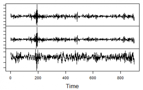
Figure 4. Components resulting from decomposition SSA
In the time series plot (Figure 3) can be seen that in such data there is a volatility of a large value over a certain period and a small value over another period. An ARIMA model was constructed for ASII stock data, resulting in ARIMA (1,1,0) as the best model. After checking the residuals, it was found that there was a heteroscedasticity effect, so a GARCH model was used for the variance model. The GARCH(1,1) model was obtained as the best variance model.
Next, we construct the SSA-ARIMA model by decomposing ASII stock data using SSA. There are two groups of components into which the series can be decomposed: the signal component and the noise component.
Figure 4 shows the decomposition of SSA components. ARIMA modeling was applied to the data after time series was decomposed using SSA to separate the signal from the noise. The noise still correlated, hence, ARIMA modeling was done on the noise. Forecasting is the total of forecasting for both signal and noise. Then the residuals were checked again and there was no longer any correlation. MAE as the accuracy value of forecasting in the ARIMA and SSA-ARIMA on the training and testing data can be seen in Table 2. The MAE value of the SSA-ARIMA model is lower than that of the ARIMA model, indicating better forecasting accuracy. Thereafter, the heteroscedasticity effect was examined using the squared residuals test for serial correlation. There was a heteroscedasticity effect, so a GARCH model was used for the variance model. The mean model's MAE decreased by around 34 percent.
Table 2. MAE value for ASII stock price
|
Model |
Training |
Testing |
|
ARIMA |
87.05 |
253.59 |
|
SSA-ARIMA (I) |
66.91 |
169.44 |
|
SSA-ARIMA (II) |
57.08 |
167.73 |
The ARIMA model for the signal is as follows:
$Y_t=Y_{t-1}+0.9541 Y_{t-1}-0.9541 Y_{t-2}+0.9972 \varepsilon_{t-1}+\varepsilon_t$ (34)
here is the ARIMA model for noise:
$\begin{gathered}Y_t=0.0555+1.0128 Y_{t-1}-0.3178 Y_{t-2}-0.0847 Y_{t-3} \\ -\varepsilon_{t-1}+\varepsilon_t\end{gathered}$ (35)
and here is the variance model:
$\sigma_t^2=144.003322+0.03489 \varepsilon_{t-1}^2+0.93818 \sigma_{t-1}^2$ (36)
After the GARCH model was established, a residual check was performed to assess whether any heteroscedasticity effects remained in the residuals. This was done using the Ljung–Box test on the squared residuals and the ARCH–LM test. Table 3 indicates that there are no remaining heteroscedastic effects in the residuals. The SSA-ARIMA-GARCH model features a larger p-value than the ARIMA-GARCH model, suggesting a reduction in the heteroscedasticity effects on the residuals. An increase of 39 percent was observed in the Ljung-Box test p-value for squared residuals from the GARCH model used to model variance.
Table 3. p-value of squared residuals Ljung-Box and ARCH-LM test for GARCH model
|
Ljung-Box Test |
|||
|
Lag |
ARIMA-GARCH |
SSA-ARIMA-GARCH (I) |
SSA-ARIMA-GARCH (II) |
|
10 |
0.54 |
0.72 |
0.75 |
|
15 |
0.42 |
0.66 |
0.70 |
|
20 |
0.30 |
0.86 |
0.89 |
|
ARCH-LM Test |
|||
|
|
0.70 |
0.83 |
0.85 |
To compare the predictive performance of the ARIMA-GARCH and SSA-ARIMA-GARCH models, the Diebold–Mariano (DM) test was conducted using the squared forecast errors as the loss function. The test yielded a DM statistic of 9.9427 with a p-value less than 2.2×10⁻¹⁶, indicating a statistically significant difference in forecast accuracy between the two models at the 1% significance level. Furthermore, the mean of the loss differential, computed as the squared error of the ARIMA-GARCH model minus that of the SSA-ARIMA-GARCH model, was positive (8648.331), suggesting that the SSA-ARIMA-GARCH model consistently produced more accurate forecasts. Therefore, it can be concluded that the SSA-ARIMA-GARCH model outperforms the ARIMA-GARCH model in terms of predictive accuracy.
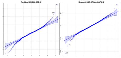
Q-Q plots of residuals (Figure 5) show that the residuals from the SSA–ARIMA–GARCH model are more normally distributed than those of the ARIMA–GARCH model, indicating an improved model fit due to the incorporation of SSA.
As shown in Figure 6, Q-Q plots of squared residuals indicate that the SSA–ARIMA–GARCH model addresses heteroskedasticity more effectively than the ARIMA–GARCH model, with squared residuals more closely resembling a normal distribution.
This study introduces a novel approach by employing SSA to handle heteroscedasticity in time series data. SSA is utilized to decompose the original series into two primary components: signal and noise. Following this decomposition, ARIMA modeling is conducted under two distinct treatments. The first treatment involves fitting the ARIMA model exclusively to the signal component, disregarding the noise. In the second treatment, ARIMA is applied to both the signal and noise components, particularly when autocorrelation is detected within the noise. If the ARIMA residuals continue to exhibit ARCH effects, the GARCH model is subsequently employed to model the conditional variance. This comprehensive strategy constitutes the hybrid SSA–ARIMA–GARCH model.
Figure 5. Q-Q plots of residuals
Figure 6. Q-Q plots of squared residuals
Time series models commonly assume constant error variance; however, financial data often exhibit heteroscedasticity. This study discusses the use of the SSA–ARIMA model for time series data exhibiting heteroscedasticity. To capture the variance of the residuals from the SSA–ARIMA approach, the GARCH model is subsequently applied—a step not addressed in previous studies. The resulting model, referred to as SSA–ARIMA–GARCH, utilizes SSA to separate the original time series into signal and noise components. In this paper, before ARIMA-GARCH modeling, decomposition is performed using SSA, where the data is decomposed into signal and noise. Two SSA-ARIMA-GARCH models are proposed in this paper. The first model ignores the noise and only models ARIMA on the signal. The second model considers both signal and noise using an ARIMA model for each, the forecast is the total of the predictions for noise and signals. This second model can be built when there is autocorrelation in the noise. In case of autocorrelation in noise, the mean absolute error of the second model is smaller than that of the first model.
The simulation data based on mean absolute error show that SSA-ARIMA-GARCH, which combines ARIMA-GARCH with SSA, is more effective than ARIMA-GARCH without SSA. Likewise for the real data, that is, ASII stock price, the mean absolute error of the mean model on with decreased by about 34 percent, and the p-value of squared residuals Ljung box test on the GARCH as variance model increased by 39 percent.
[1] Engle, R.F. (1982). Autoregressive conditional heteroscedasticity with estimates of the variance of United Kingdom inflation. Econometrica, 50(4): 987-1007. https://www.jstor.org/stable/1912773.
[2] Bollerslev, T. (1986). Generalized autoregressive conditional heteroscedasticity. Journal of Econometrics, 31(3): 307-327. https://doi.org/10.1016/0304-4076(86)90063-1
[3] Enders, W. (2014). Applied Econometrics Time Series. John Wiley & Sons Inc.
[4] Paolella., M.S. (2019). Linear Models and Time-Series Analysis: Regression, ANOVA, ARMA, and GARCH. John Wiley & Sons Ltd. https://doi.org/10.1002/9781119432036
[5] Abreu, R.J., Souza, R.M., Oliveira, J.G. (2019). Applying singular spectrum analysis and ARIMA-GARCH for forecasting EUR/USD exchange rate. Revista de Administração Mackenzie, 20(4): 1-32. https://doi.org/10.1590/1678-6971/eRAMF190146
[6] Hassani, H., Thomakos, D. (2010). A review on singular spectrum analysis for economic and financial time series. Statistics and Its Interface, 3(3): 377-397. https://doi.org/10.4310/SII.2010.v3.n3.a11
[7] Sulandari, W., Subanar, Suhartono, Utami, H., Lee, M.H. (2018). An empirical study of error evaluation in trend and seasonal time series forecasting based on SSA. Pakistan Journal of Statistics and Operation Research, 14(4): 945. https://doi.org/10.18187/pjsor.v14i4.2443
[8] Safitri, D., Subanar, Utami, H., Sulandari, W. (2019). Forecasting of Jabodetabek train passengers using singular spectrum analysis and holt-winters methods. Journal of Physics: Conference Series, 1524: 012100. https://doi.org/10.1088/1742-6596/1524/1/012100
[9] Sulandari, W., Yudhanto, Y., Rodrigues, P.C. (2022). The use of singular spectrum analysis and K-means clustering-based bootstrap to improve multistep ahead load forecasting. Energies, 15(16): 5838. https://doi.org/10.3390/en15165838
[10] Oliveira Santos, M.F., Souza, R.M., Corrêa, W.L.R. (2024). Singular spectrum analysis to estimate core inflation in Brazil. Central Bank Review, 24(4): 100177. https://doi.org/10.1016/j.cbrev.2024.100177
[11] Elsner, J.B. (2002). Analysis of time series structure: SSA and related techniques. Journal of the American Statistical Association, 97(460): 1207-1208. https://doi.org/10.1198/jasa.2002.s239
[12] Golyandina, N., Zhigljavsky, A. (2013). Singular Spectrum Analysis for Time Series. Springer. https://doi.org/10.1007/978-3-642-34913-3
[13] Degiannakis, S., Filis, G., Hassani, H. (2018). Forecasting global stock market implied volatility indices. Journal of Empirical Finance, 46: 111-129. https://doi.org/10.1016/j.jempfin.2017.12.008
[14] Golyandina, N., Nekrutkin, V., Zhigljavsky, A.A. (2001). Analysis of Time Series Structure: SSA and Related Techniques. Chapman and Hall/CRC, New York. https://doi.org/10.1201/9780367801687
[15] Hassani, H. (2007). Singular spectrum analysis: Methodology and comparison. Journal of Data Science, 5(2): 239-257. https://doi.org/10.6339/JDS.2007.05(2).396
[16] Golyandina, N., Korobeynikov, A. (2014). Basic singular spectrum analysis and forecasting with R. Computational Statistics & Data Analysis, 71: 934-954. https://doi.org/10.1016/j.csda.2013.04.009
[17] Sulandari, W., Subanar, Lee, M.H., Rodrigues, P.C. (2020). Time series forecasting using singular spectrum analysis, fuzzy systems and neural networks. MethodsX, 7: 101015. https://doi.org/10.1016/j.mex.2020.101015
[18] Sulandari, W., Subanar, S., Lee, M.H., Rodrigues, P.C. (2020). Indonesian electricity load forecasting using singular spectrum analysis, fuzzy systems and neural networks. Energy, 190: 116408. https://doi.org/10.1016/j.energy.2019.116408
[19] Sulandari, W., Subanar, Suhartono, Utami, H., Lee, M.H., Rodrigues, P.C. (2020). SSA-based hybrid forecasting models and applications. Bulletin of Electrical Engineering and Informatics, 9(5): 2178-2188. https://doi.org/10.11591/eei.v9i5.1950
[20] Suhartono, Isnawati, S., Salehah, N.A., Prasetyo, D.D., Kuswanto, H., Lee, M.H. (2018). Hybrid SSA-TSR-ARIMA for water demand forecasting. International Journal of Advances in Intelligent Informatics, 4(3): 238-250. https://doi.org/10.26555/ijain.v4i3.275
[21] Irmawati, D.R., Atok, R.M., Suhartono. (2018). Hybrid singular spectrum analysis-ARIMA modelling for direct and indirect forecasting of Farmer's Term of Trade in East Java. In 2018 International Conference on Information and Communications Technology (ICOIACT), Yogyakarta, Indonesia, pp. 889-894. https://doi.org/10.1109/ICOIACT.2018.8350823
[22] Arteche, J., Garcia-Enriquez, J. (2022). Singular spectrum analysis for value at risk in stochastic volatility models. Journal of Forecasting, 41(1): 3-16. https://doi.org/10.1002/for.2796
[23] Hassani, H., Alharbi, N., Ghodsi, M. (2014). A short note on the pattern of singular values of scaled random Hankel matrix. International Journal of Applied Mathematics, 27(3): 237-243. https://doi.org/10.12732/ijam.v27i3.4
[24] Wei, W.W.S. (2006). Time Series Analysis: Univariate and Multivariate Methods. Pearson Addison Wesley.
[25] Brockwell, P.J., Davis, R.A. (2016). Introduction to Time Series and Forecasting. Springer, pp. 157-164. https://doi.org/10.1007/978-3-319-29854-2
[26] Tsay, R.S. (2010). Analysis of Financial Time Series. John Wiley & Sons Inc. https://doi.org/10.1002/9780470644560
[27] Francq, C., Zakoïan, J.M. (2010). GARCH Models: Structure, Statistical Inference and Financial Applications. John Wiley & Sons Ltd. https://doi.org/10.1002/9780470670057
[28] Neusser, K. (2016). Time Series Econometrics. Springer, pp. 173-184. https://doi.org/10.1007/978-3-319-32862-1