Impact of Equilibration Steps on Quantum Monte Carlo for the Spin-1/2 Heisenberg Model

The spin-lattice model is a mathematical framework used to study interacting spins arranged on a lattice, representing quantum systems like magnets [1]. These models are described using Hamiltonians, which capture spin interactions and quantum properties and are often explored through analytical methods (e.g., Bethe ansatz) or numerical techniques (e.g., Monte Carlo) [2]. Spin lattice models are crucial for understanding quantum phenomena like phase transitions and entanglement. The Stochastic Series Expansion (SSE) method efficiently handles these models by directly sampling the partition function's power series, avoiding discretization errors and enabling precise simulations of thermodynamic properties [3, 4].

The SSE method is a very efficient quantum Monte Carlo (QMC) technique widely used in simulating quantum systems at finite temperatures [5-7]. This method is valuable in studying complex quantum phenomena, especially in low-dimensional and strongly correlated systems [8]. SSE leverages Taylor series expansion on the partition function of the system combined with nonlocal Monte Carlo updates [9], allowing direct sampling of the partition function expansion in powers of the Hamiltonian. This capability enables SSE to accurately simulate the thermodynamic properties of quantum spin systems, which is crucial in understanding quantum phase transitions and magnetic properties. This approach avoids the errors associated with time discretization [10].

An important factor in the development of QMC techniques has been Feynman's path integral formulation of quantum statistical mechanics [11]. World-line methods are frequently used to refer to techniques based on the path integral in imaginary time in the context of spin systems and related lattice models [12, 13]. The methods began by using an approximation discretization of imaginary time, known as the Suzuki-Trotter decomposition of the Boltzmann operator $e^{-\beta \hat{H}}; \beta$ is the inverse dimensionless temperature. Such methods often introduce systematic errors due to discretization [14]; such errors arise because discrete jumps approximate the continuous dynamics of the system. This means that the true nature of quantum fluctuations is not fully captured. Additionally, Trotter-Suzuki Approximation Errors, a systematic error occurs because of splitting the exponential of a sum of operators into a product of exponentials [15, 16], each involving smaller time steps. This error decreases with the square of the time steps; however, achieving high-accuracy simulation requires smaller time steps, which increases the computational cost. SSE effectively avoids such errors by directly expanding the partition function in terms of a power series of the Hamiltonian operators with discretizing. Furthermore, SSE does not require Trotter-Suzuki approximations [10]. The progress in the QMC algorithm has mainly been made in two areas: (a) by removing the systematic error found in the Trotter decomposition and (b) by creating loop-cluster algorithms to enable efficient sampling inside the configuration space of quantum systems. SSE is a generalization of Handscomb’s QMC scheme, which combines (a) and (b) with even more speedups for SSE’s loop-cluster algorithms. Such speedups provide a shorter time for autocorrelation than other methods, enabling the studies of larger system sizes [17, 18].

Monte Carlo steps play various critical roles in the SSE method. They ensure the accuracy of sampling configuration space and that the results represent the true equilibrium properties of the system. Monte Carlo steps bring the system into thermal equilibrium in the first phase of the simulation, allowing the system to reach a steady state where the sampled configurations represent the system’s equilibrium distribution [19, 20].

Monte Carlo steps used in equilibration [21] are termed ($i_{\text {steps}}$) in this paper. Proper equilibration provides unbiased results when measurements are taken. Furthermore, each step of Monte Carlo simulation proposes an accept or reject of the new configuration of the system based on a probabilistic criterion; typically, Metropolis and other algorithms are used in this process. Efficient sampling ensures that all simulated configurations are considered according to their Boltzmann weights, accurately estimating physical quantities, such as energy, magnetization, and susceptibility. Monte Carlo steps are also used in diagonal and loop updates. The term used to refer to the Monte Carlo steps taken while measuring system properties is $M_{\text {steps}}$ (i.e., measurements taken after the system has reached equilibrium). One bin represents the average of all individual results obtained at each $M_{\text {steps}}$.

This paper studies the impact of Monte Carlo steps used for equilibration on the computational cost, stability, and feasibility of SSE results for various properties, including ground state energy, sublattice magnetization, specific heat, and susceptibility for different lattice sizes and temperatures.

This work aims to investigate the impact of $i_{\text {steps}}$ on the accuracy, stability, and computational efficiency of the SSE simulations, particularly for the 1D Heisenberg mode. The motivation stems from the crucial role equilibration plays in ensuring that Monte Carlo simulations correctly sample the equilibrium state of a quantum system. While significant progress has been made in understanding Monte Carlo methods and their applications, systematic studies quantifying the relationship between $i_{\text {steps}}$, physical observables, and computational costs remain limited.

The study commences with an overview of the foundational formulation of the SSE method, including the mathematical framework underpinning this approach. Subsequently, the results and discussion section present an analysis of the simulation outcomes, focusing on computational cost, magnetic properties of the system, and data convergence. The paper also provides a guide for researchers on selecting appropriate simulation parameters to ensure reliable results. The study's limitations are then outlined, followed by a concluding section summarizing the key findings of the research.

The simulation of 1D spin-1/2 antiferromagnetic system defined by the Heisenberg model using SSE was analyzed to explore the effect of $i_{\text {steps}}$ on the system's physical properties, including ground state energy per spin ($E_0 / N$), specific heat $(C)$, sublattice magnetization $\left(\left\langle m^2\right\rangle\right)$, and susceptibility $(\chi)$. The simulations were implemented in FORTRAN90, utilizing the Sandvik algorithm to perform the SSE calculations [26]. The computational work was executed on a personal computer equipped with an AMD Ryzen 7 3700X 8-Core Processor (3.60 GHz) and 16 GB of G. Skill Radiant 3600 MHz RAM, ensuring the capability to handle the significant computational demands of the study. We first present the computational cost for a range of temperatures and $i_{\text {steps}}$. Furthermore, the study investigates the stability of the simulation outcomes for different temperatures and multiple $i_{\text {steps}}$ counts. Additionally, the same conditions but changing the steps were conducted to examine if the technique returned converged results and also for a range of temperatures. In this study, also we performed simulations on relatively large systems and low temperatures to examine the effectiveness of SSE on complex conditions.

3.1 Computational cost

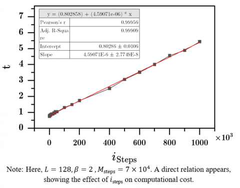
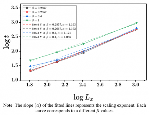
This study investigates the impact of $i_{\text {steps}}$ on processing time and found that they have a significant effect. It's clear that processing time increases as the number of $i_{\text {steps}}$ increases, as shown in Figure 1. It's worth noting that even if there are zero $i_{\text {steps}}$, the processing time is not zero, as $M_{\text {steps}}$ also require some time. However, the equilibration of a system with a relatively high temperature is achieved faster than a low-temperature one. The processing time scales approximately with lattice size $t \propto L^\alpha$, where $\alpha$ is the slope of each fitted line in Figure 2. The scaling exponents are above 1 for all $\beta$ indicating that the processing time grows faster than a linear scaling, reflecting the increased computational cost required to handle larger systems. At lower temperatures, the processing time grows more rapidly with lattice size. While it takes less time for higher temperatures (lower $\beta$), this can be seen from the smaller $\gamma$ of $\beta=1.0$, indicating slower growth of processing time with lattice size. This behavior is due to the slower equilibration in low temperatures with more pronounced quantum effects.

From the fitting of plots of processing time ($t$) with simulation parameters, $t$ scales as:

$\begin{gathered}t\left(L, \beta, M_{\text {steps}}, i_{\text {steps}}\right)=L^\alpha \cdot \beta^\gamma \cdot M_{\text {steps}}^\delta \cdot 10^{B_2\left(\log i_{\text {steps}}\right)^2+B_1 \log i_{\text {steps}}+B_0}\end{gathered}$          (13)

where, $B_1, B_2$ and $B_0$ are the polynomial coefficients from the $\log -\log$ fitting of $i_{\text {steps}}$, and $\alpha, \gamma$, and $\delta$ are the scaling exponents derived from the other parameters, each one of these coefficients is shown in the following figures and will be discussed individually.

1.png

Figure 1. Relation between $i_{\text {steps}}$ and time in seconds

2.png

Figure 2. Log-log plot of processing time $(t)$ versus lattice size ($L$) for various values of $\beta$, with $M_{\text {steps}}=10^6$ and $i_{\text {steps}}=10^4$

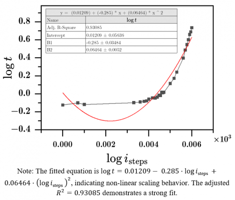
We can see that $t$ exhibits district scaling behavior with various simulation parameters. Figure 2 demonstrates the power law relationship between time and lattice size, where $\alpha$ vary slightly with $\beta$. This highlights that computational cost increases with system size due to larger configurations requiring more extensive calculations. Figure 3 presents the relationship between processing time and $i_{\text {steps}}$. Here we applied a second-degree polynomial fitting to capture the nonlinear trend. For small values of $i_{\text {steps}}$, the negative linear term $\left(-0.285 \cdot \log i_{\text {steps}}\right)$ leads to a decrease in the processing time, but rapid growth for larger $i_{\text {steps}}$ is observed in the term $\left(0.06464 \cdot\left(\log i_{\text {steps}}\right)^2\right)$ which causes a sharp increase in $t$. The nonlinear scaling underscores the importance of carefully selecting $i_{\text {steps}}$ to balance computational cost and accuracy.

3.png

Figure 3. Log-log plot of processing time versus $i_{\text {steps}}$ with a second-degree polynomial fit

4.png

Figure 4. Log-log plot of processing time versus the number of $M_{\text {steps}}$ for a fixed $L, i_{\text {steps}}, \beta$

5.png

Figure 5. Log-log plot of processing time versus inverse temperature $(\beta)$ for a lattice size $L=128, M_{\text {steps}}=10^6$, and $i_{\text {steps}}=10^4$

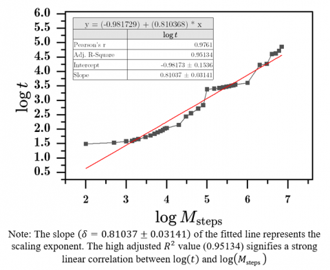
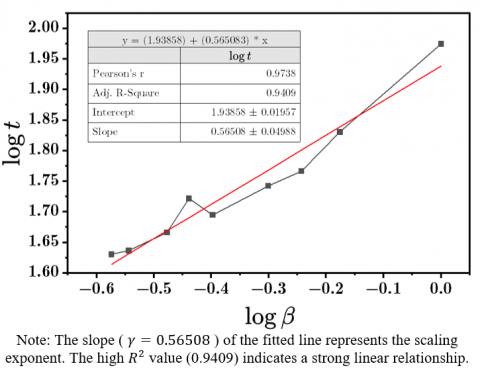
Figure 4 shows that time scales with $M_{\text {steps}}$ with scaling exponent $\delta=0.81037$, indicating sublinear growth, thus reflecting the computational efficiency of averaging over repeated steps. In Figure 5, the processing time increases modestly as $\beta$ increases with the scaling exponent ($\gamma=$ 0.565). The inverse temperature ($\beta$) influences the level of thermal fluctuations in the system, higher $\beta$ values require more computational effort to accurately sample the configuration space and achieve equilibration.

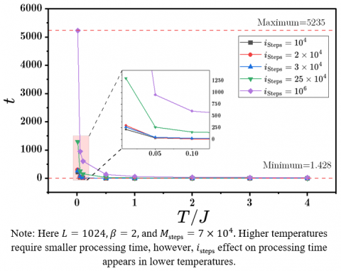
Figure 6 shows that lower temperatures (where the quantum phenomena are dominant) require longer processing time. Yet the effect of equilibration $i_{\text {steps}}$ is obvious for lower temperatures, too. Thus 10⁴ $i_{\text {steps}}$ took 222 seconds but more than 5000 seconds were taken for 10⁶ $i_{\text {steps}}$ for the same temperature. On the other hand, the processing time of all five cases of $i_{\text {steps}}$ was the same for higher temperatures., i.e., they required fewer equilibration steps.

6.png

Figure 6. Processing time in seconds for a range of dimensionless temperatures, for multiple $i_{\text {steps}}$

3.2 Magnetic properties with different $\boldsymbol{i}_{\text {steps}}$

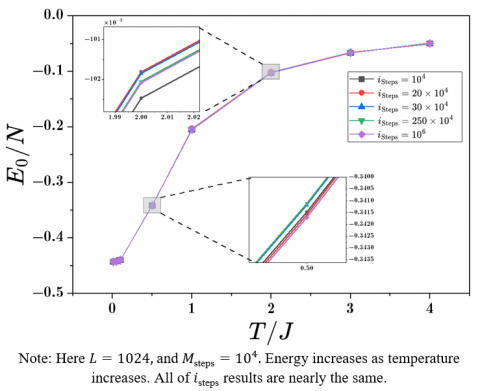
We investigated the outcomes of different system properties in various temperatures and for different cases of $i_{\text {steps}}$. Ground state energy of quantum spin-1/2 chain increases with temperatures, as shown in Figure 7. A match of all the outcomes is noticed for all the $i_{\text {steps}}$ cases, indicating that the studied system's equilibration reached all $i_{\text {steps}}$ counts, and the results were nearly the same. We can see from Table 1 that the standard deviation $(\sigma)$ is larger for lower number of $i_{\text {steps}}$, and the results deviate from the exact solution. By using a low temperature $(\beta=64)$, the system approaches the zerotemperature limit, allowing the results to approximate the exact ground-state energy per spin calculated using the Bethe ansatz, which is defined for absolute zero temperature [27].

7.png

Figure 7. Ground state energy relation with the dimensionless temperature at a range of $i_{\text {steps}}$

8.png

Figure 8. The relation between sublattice magnetization and dimensionless temperatures, each point simulated in multiple counts of $i_{\text {steps}}$

9.png

Figure 9. Susceptibility versus dimensionless temperature for different $i_{\text {steps}}$ counts

The magnetization shows higher values at low temperatures (see Figure 8), reflecting strong correlation between spins. As the temperature increases, thermal fluctuations dominate, leading to a gradual decrease in the property. The result is consistent across different $i_{\text {steps}}$, i.e., the system reaches equilibrium and is not influenced by varying $i_{\text {steps}}$.

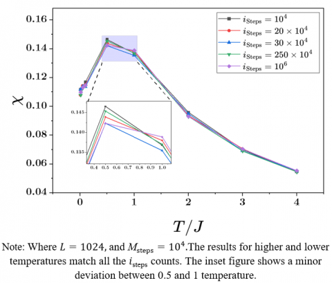
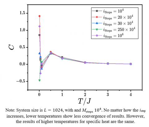
The susceptibility peaks at intermediate temperatures as shown in Figure 9, representing the formation of short-range correlations. In such temperatures, the system transitions into the Curie-Weiss behavior [28,29] due to the paramagnetic response of spins. The inset shows minor differences at low $i_{\text {steps}}$, but the overall trend is consistent across different equilibration steps. In the case of specific heat, Figure 10 shows that at low temperatures, smaller $i_{\text {steps}}$ introduce greater fluctuations, indicating insufficient equilibration. As temperature increases, $C$ aligns across all $i_{\text {steps}}$. At $T / J=0.5$, the specific heat reflects the Schottky-like anomaly, associated with thermal excitations between spin states. At higher temperatures, $C$ approaches a constant value, reflecting equipartition.

10.png

Figure 10. Specific heat for a range of dimensionless temperatures and various $i_{\text {steps}}$

In Table 1, the lattice size $L=128, \beta=1 / 64$, and $M_{\text {steps}}=10^4$. Insufficient $i_{\text {steps}}$ lead to results that have a larger $\sigma$ and deviate from the exact solution obtained via Beth Ansatz.

Table 1. Standard deviation $(\sigma)$ of energy results for various $i_{\text {steps}}$, calculated with $N_{\text {bins}}=10$

Table 2 lists the average values $\langle X\rangle$, standard deviation ($\sigma$), variance ($\sigma^2$), and relative deviation ($\sigma /\langle X\rangle$) for each observable. The results demonstrate that $i_{\text {steps}}$ does not significantly influence the convergence of data across multiple simulation runs, as evidenced by the relatively constant standard deviation and variance.

Table 2. Statistical analysis of observables as a function of $i_{\text {steps}}$

3.3 Results accuracy and convergence

Measurements in the SSE method are taken after the equilibration is reached. Several $i_{\text {steps}}$ are used for this purpose. However, those steps take time, as discussed above. A threshold of $i_{\text {steps}}$ can be calculated for the system of investigation where the results remain similar regardless of the number of $i_{\text {steps}}$ added; Figure 11 shows that insufficient $i_{\text {steps}}$ count gives inaccurate outcomes as in the incent Figure 11(a), the energy in the first two points of the data doesn't represent the actual value of the system. Conversely, more elevated $i_{\text {steps}}$ give the same results; Higher $M_{\text {steps}}$ count reduces error bars as appears in Figure 11(b). The data in Table 2 clearly show that $i_{\text {steps}}$ does not govern the convergence of the results from multiple runs of simulation, as $\sigma$ and $\sigma^2$ remains largely unchanged across different $i_{\text {steps}}$. This also indicates that the convergence of data is the responsibility of $M_{\text {steps}}$ which ensures proper sampling and reduces variability across runs. Nevertheless, $i_{\text {steps}}$ is crucial for the accuracy of results. Proper $i_{\text {steps}}$ ensures that the system is equilibrated and the measurements reflect the true magnetic behavior of the system. This highlights the roles of $M_{\text {steps}}$ and $i_{\text {steps}}$ in achieving both convergence and accuracy in the simulation data.

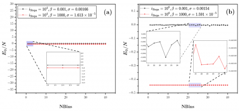
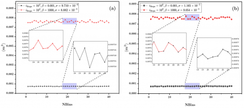
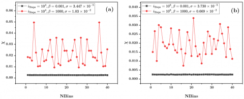
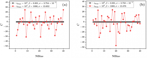
We represent from Figures 12-15 a repeated simulation results for the same conditions and two different values of $i_{\text {steps}}$ to assess the reliability and consistency of the simulation outcomes. These figures highlight the impact of varying $i_{\text {steps}}$ under extreme temperature, both very high and very low, on the studied magnetic properties.

In Figure 12, $E_0 / N$ demonstrates consistent results across 40 simulation runs for both low and high temperatures. However, at low $i_{\text {steps}}$ (Figure 12(a)) the energy values for high and low temperatures appear nearly identical, suggesting that the system has not yet reached equilibrium. But the higher $i_{\text {steps}}$ in Figure 12(b), the high temperature simulations yield higher energy values as expected from real magnetic system, indicating improved precision.

12.png

Figure 12. Results of energy for 40 runs of the same simulation for low and high temperatures with (a) $10^4$ and (b) $10^6 i_{\text {steps}}$, where $L=1024$, and $M_{\text {steps}}=10^4$

13.png

Note: The property has a reverse relation with temperature. And it converges more for higher temperatures.

Figure 13. Simulation outcomes of sublattice magnetization for low and high temperatures for a system with $L=1024$ spin sites. Each NBin results from averaging $10^4 M_{\text {steps}}$, after equilibrating the system by (a) $10^4$ and (b) $10^6 i_{\text {steps}}$

14.png

Note: Results of higher temperatures shows less standard deviation $\sigma$.

Figure 14. Susceptibility results for $40 N_{\text {Bins}}$, for system size $L=1024$, at each point, susceptibility was measured by averaging the results of $10^4 M_{\text {steps}}$ after (a) $10^4$ and (b) $10^6$ equilibration Monte Carlo steps

15.png

Note: Lower temperatures (i.e. higher $\beta$) show major fluctuations of results.

Figure 15. Specific heat of $L=1024$, where $M_{\text {steps}}=10^4$, each point represents on run of simulation at low and high temperatures, the $i_{\text {steps}}$ was (a) $10^4$ and (b) $10^6$

16.png

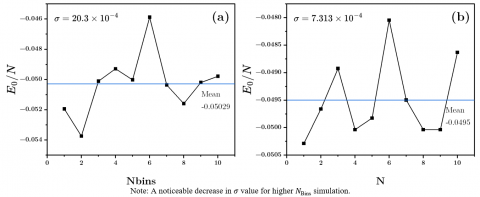
Figure 16. Repeating the simulation of the same conditions where $L=64, \beta=0.25$, and $M_{\text {steps}}=i_{\text {steps}} v=10^4$, each point in the figure represents (a) 1 and (b) $10 N_{\text {Bins}}$

$\left\langle m^2\right\rangle$ shows higher values and larger standard deviations at lower temperatures (see Figure 13), consistent with the expected stronger ordering in the system. Figure 13(a) and (b) both display reliable results across repeated simulations, thus increase in the $i_{\text {steps}}$ does not significantly affect the outcomes. The results of specific heat and susceptibility, shown in Figure 14 and Figure 15, exhibit more pronounced temperature dependence. At low temperature, the red data points in Figure 14(a) and (b) oscillate within a wider range (0.01 to 0.05 for $\chi$), reflecting the challenge of achieving precise convergent in this regime. Higher temperature simulations (black data points) remain relatively stable, with minimal influence from $i_{\text {steps}}$. Similar for $C$, low-temperature results show significant fluctuations, while high temperatures yield consistent outcomes (Figure 15). We can notice that increasing $i_{\text {steps}}$ from $10^4$ to $10^6$ does not significantly alter the results for $C$, thus the convergence for this property is not governed by $i_{\text {steps}}$. Figure 16 demonstrates the effect of averaging over multiple bins on the stability and reliability of the simulation results for the ground state energy per spin, where $N_{\text {bins}}=10$ in Figure 16(a), the data shows a higher standard deviation ( $\sigma= 20.3 \times 10^{-4}$), By increasing the $N_{\text {bins}}$ to 100 (see Figure 16(b)), $\sigma$ significantly decreases to $7.31 \times 10^{-4}$, reflecting a more stable and consistent set of results. The reduced variability for higher $N_{\text {bins}}$ ensures greater confidence in the accuracy of the reporter results.

3.4 Criteria for determining appropriate $i_{\text {steps}}$

The accuracy and stability of SSE simulations are contingent upon selecting an adequate number of equilibration steps ($i_{\text {steps}}$). We outline a systematic frame work for determining the optimal $i_{\text {steps}}$.

1. Preliminary Investigations:

Initial trail simulations should be conducted across a range of $i_{\text {steps}}$ to identify the equilibration threshold. Key observables, such as $E_0 / N$ and $\left\langle m^2\right\rangle$ should be monitored for evidence of stabilization. If a plateau appears in these observables, then the system has reached equilibrium.

2. Autocorrelation Analysis:

The auto correlation time of critical observables provides a quantitative measure of the statistical independence between successive configurations. $i_{\text {steps}}$ should must exceed the auto correlation time by a factor at least 10 .

3. Statistical Validation:

To ensure robust equilibration, the stability of statistical measures such as the mean and variance of observables should be evaluated. Convergence is achieved when the mean value stabilizes within a predefined tolerance and the variance exhibits no significant dependence on $i_{\text {steps}}$.

It is noted that higher temperatures may diminish the requisite number of $i_{\text {steps}}$ for equilibration, whereas larger systems typically necessitate an increased number of $i_{\text {steps}}$. Statistical methods should be employed to ascertain the stabilization of the mean and variance of the measurements, thereby ensuring robust and reliable simulation outcomes.

This study examines the role of equilibration steps in the SSE method for simulating the 1D spin-1/2 antiferromagnetic lattice defined by the Heisenberg model. The findings highlight the critical importance of equilibration steps in achieving stable and reliable simulation outcomes while balancing computational cost. The analysis demonstrates that ground state energy per spin and sublattice magnetization remain stable across different equilibration step counts, particularly at low temperatures, closely matching the exact Bethe ansatz solution. In contrast, susceptibility and specific heat show variability at low temperatures due to dominant quantum effects. At intermediate temperatures, susceptibility peaks reflect the formation of short-range spin correlations and transition into Curie-Weiss behavior at high temperatures. The results also emphasize that increasing the number of bins significantly enhances result stability by reducing statistical deviations.

Equilibration steps are vital to ensure accurate representation of the system’s equilibrium properties, particularly at low temperatures where slower equilibration leads to greater fluctuations. Measurement steps, on the other hand, govern the convergence of results across multiple runs, ensuring proper sampling and consistency.

Future work could explore these findings in higher-dimensional systems, ladder geometries, or more complex spin interactions. An automated algorithm could be developed to optimize simulation parameters, such as equilibration and measurement steps, based on the system's properties, including lattice size and temperature. The algorithm would perform several preliminary runs to analyze the system's behavior and identify the optimal values for equilibration and measurement steps that ensure both accuracy and computational efficiency. Additionally, the algorithm could factor in the hardware specifications of the system it is running on, such as the processor type, available RAM, and computational power. The algorithm could adapt to hardware capabilities, efficiently allocating resources and recommending parameters that balance accuracy and runtime. This automation would save time, especially for larger lattices or low temperatures, reducing trial-and-error and enabling researchers to focus on analyzing results.