Inaam Rikan Hassan*![]() | Poh Soon JosephNg
| Poh Soon JosephNg![]() | Felix Pasila
| Felix Pasila![]()
© 2025 The authors. This article is published by IIETA and is licensed under the CC BY 4.0 license (http://creativecommons.org/licenses/by/4.0/).
OPEN ACCESS
Selective Harmonic Elimination Pulse Width Modulation (SHE-PWM) is an effective but complex modulation technique in power electronics, requiring solutions to nonlinear equations. Solving these equations is a challenging optimization problem that demands high accuracy and significant computational effort. This study introduces the multi-strategy improved parrot optimization (MPO) algorithm to solve the nonlinear SHE equations for an 11-level inverter. The performance of the MPO algorithm is compared with classical and modern optimization techniques, including Newton-Raphson (NR), Differential Evolution (DE), Genetic Algorithm (GA), Particle Swarm Optimization (PSO), and Parrot Optimizer (PO). The results demonstrate that MPO outperforms these methods in terms of solution quality and convergence speed. Evaluations were conducted using a suite of benchmark functions, highlighting the practical advantage of MPO as a reliable and efficient tool for optimization in SHE-PWM applications and other power electronics modulation problems.
mathematical modeling, solution of nonlinear equations, Pulse Width Modulation (PWM), Selective Harmonic Elimination (SHE), metaheuristic algorithms, multi-strategy parrot optimization, optimization techniques
Nonlinear equations, often characterized by variables raised to varying powers or involved in multiplicative interactions, are central to modeling complex systems in engineering, physics, and applied mathematics. These equations frequently exhibit multiple equilibria, bifurcations, and chaotic behavior, presenting significant analytical and numerical challenges [1, 2]. The solution of such equations is important to the accurate modeling of phenomena such as electrical circuit behavior, fluid dynamics, and nonlinear control systems. Most nonlinear equations cannot be solved by conventional methods of analysis, as there are no closed-form solutions. Consequently, there has been extensive use of iterative numerical methods, which include the Newton-Raphson (NR) method. Although NR can converge towards roots quadratically, its convergence may not work well in the case of an ill-conditioned Jacobian matrix or highly non-convex problems, in that a bad initial guess can lead to divergence, or a poor guess may produce unwanted answers even when this algorithm converges [3, 4].
To answer these solutions, heuristic and metaheuristic population-based optimization algorithms have become of great importance. Such derivative-free algorithms have also been successfully used with nonlinear optimization problems because they possess a powerful global search behavior and have the intrinsic avoidance of local optima traps. An example is the Differential Evolution (DE), which is a very powerful evolutionary algorithm capable of preserving the diversity of the population and also searching the continuous spaces effectively [5, 6]. In the same vein, another method well established in performing non-linear tasks optimization is Genetic Algorithms (GA) and Particle Swarm Optimization (PSO), which may be utilized in Selective Harmonic Elimination-Pulse Width Modulation (SHE-PWM) problems. Nonetheless, regarding the SHE-PWM problems, there are shortcomings related to GA and PSO, including early convergence, premature convergence, and stagnation, as well as the high computational load that the methods can require [7, 8].
The optimisation algorithm Parrot Optimisation (PO), which incorporates social actions of parrots as an inspiration, provides a novel usage of nonlinear optimization. This dynamic communication and foraging enable PO to journey through complex, multimodal search spaces optimally because they achieve the required balance between exploration and exploitation. Nonetheless, PO suffers from some of the other difficulties too, including premature convergence and the trapping of local optima, particularly on highly nonlinear and locked-up issues like the SHE-PWM [9].
In order to overcome these drawbacks, an algorithm called multi-strategy improved parrot optimization (MPO) was invented. MPO is a hybrid method that integrates several adaptive methods, including dynamic parameter adjustments, opposition-based learning, and Levy flight algorithms to enhance the trade-off between exploration and exploitation. This improvement enables MPO to keep the population diversity, prevent premature stagnation, and converge faster to make it a good choice to solve complex nonlinear SHE equations in the multilevel inverter systems [10].
The originality of the work is the use of the MPO algorithm to solve the SHE-PWM problem, for which its performance has been compared with other methods such as the GA, PSO, and PO. The MPO algorithm provides a more efficient and reliable optimization tool to manage the nonlinearities and constraints of multilevel inverter modulation. This paper fills the said gaps in research because it proves that MPO is more effective than other optimization algorithms in solving a problem, its rate of convergence, and its efficiency in computation time [11]. Therefore, this work is not just another optimization method of SHE-PWM applications but also part of the power electronics nonlinear optimization as well. In the following section, the methodology applied in this work will be outlined, including the algorithms that were tested, along with corresponding procedures of benchmarking.
The SHE-PWM is an advanced modulation technique that is widely used in an effort to enhance the output voltage characteristics of multilevel inverters [12]. Using exact calculation of switching angles in a basic half-cycle, SHE-PWM is intended to eradicate certain low-order harmonics at the inverter output to keep total harmonic distortion to a minimum without the use of large passive filtering elements. SHE-PWM is the modernized modulation approach that has been widely adopted to enhance the quality of the output voltage in a multilevel inverter. Through the accurately calculated switching angles within any given half-cycle, SHE-PWM attempts to remove certain low-order harmonics in an inverter output and hence limit total harmonic distortion without the need for large passive filters [12]. The types of SHE-PWM waveforms recorded in the literature are very many, with the stepped type being the highest in terms of implementation in the multilevel inverters [13-18]. The specified waveform is particularly used to synthesize the signal at the output that can already take the form of a sinusoid with the fail-safe reduction of a low-order harmonic distortion [19]. Figure 1 shows an example of the output voltage waveform of one phase of an 11-level three-phase multilevel inverter.
Figure 1. Voltage waveform generated by SHE-PWM in an 11-level multilevel inverter
A multilevel inverter output voltage is a nonlinear periodic signal that can be broken down into its frequency components by the Fourier series. The Fourier series expression of a periodic function $v(t)$ is denoted in Eq. (1):
$v(t)=a_0+\sum_{n=1}^{\infty}\left[a_n \cos (n \omega t)+b_n \sin (n \omega t)\right]$ (1)
where, ω=2πf is the fundamental angular frequency. The coefficients and bn represent the amplitudes of the cosine and sine harmonics, respectively. In the context of SHE-PWM, the inverter output waveform commonly exhibits half-wave symmetry and other symmetries that reduce the harmonic content to only odd harmonics, simplifying the Fourier representation.
For an 11-level inverter, the output waveform within one quarter cycle is defined by five switching angles $\theta_1$ to $\theta_5$, subject to the constraints of Eq. (2):
$0 \leq \theta_1<\theta_2<\theta_3<\theta_4<\theta_5 \leq \frac{\pi}{2}$ (2)
These switching angles determine the instant at which the inverter output changes its voltage level, Eq. (3). The amplitude of the nth harmonic component of the output voltage can be expressed as Eq. (4):
$V_n=\frac{4 V_{d c}}{n \pi} \sum_{k=1}^5(-1)^{k+1} \cos \left(n \theta_k\right)$ (3)
$\mathrm{THD}=\frac{\sqrt{\sum_{n=2}^{\infty} V_n^2}}{V_1}$ (4)
where, Vn is the magnitude of the nth harmonic, Vdc is the DC link voltage, n is the harmonic order (odd integers), and $\theta_k$ is the switching angle. The primary goal in SHE-PWM is to ensure that:
•The fundamental harmonic V1matches the desired reference voltage Vref .
•Specific lower-order harmonics (commonly the 5th, 7th, 11th, and 13th) are eliminated, i.e., their amplitudes are zero.
This leads to a nonlinear system of transcendental equations: Eq. (5).
The modulation index m is a key parameter that defines the fundamental output voltage amplitude relative to the DC bus voltage; it is given by the ratio of the desired fundamental peak voltage V1p to the total DC input voltage, as expressed mathematically in Eq. (6).
$\begin{aligned} & \frac{4 V_{d c}}{\pi} \sum_{k=1}^5(-1)^{k+1} \cos \left(\theta_k\right)=V_{\text {ref }} \\ & \frac{4 V_{d c}}{5 \pi} \sum_{k=1}^5(-1)^{k+1} \cos \left(5 \theta_k\right)=0 \\ & \frac{4 V_{d c}}{7 \pi} \sum_{k=1}^5(-1)^{k+1} \cos \left(7 \theta_k\right)=0 \\ & \frac{4 V_{d c}}{11 \pi} \sum_{k=1}^5(-1)^{k+1} \cos \left(11 \theta_k\right)=0 \\ & \frac{4 V_{d c}}{13 \pi} \sum_{k=1}^5(-1)^{k+1} \cos \left(13 \theta_k\right)=0\end{aligned}$ (5)
$m=\frac{V_{1 p}}{k V_{D C}}$ (6)
To quantify the harmonic content of the inverter output voltage, the Total Harmonic Distortion (THD) is used. THD is defined as the ratio of the root mean square (RMS) of all harmonic components to the RMS value of the fundamental component: V1 is the RMS amplitude of fundamental harmonics; Vn are the RMS amplitudes of the higher-order harmonics (n=2, 3…).
A lower THD value indicates better waveform quality and reduced harmonic distortion. Selective Harmonic Elimination PWM focuses on removing specific low-order harmonics, resulting in the concept of Error-based Total Harmonic Distortion (THDe), which measures the distortion from the eliminated harmonics only. It is expressed as Eq. (7):
$\mathrm{THD}_e=\frac{\sqrt{\sum_{n \in H_e} V_n^2}}{V_1}$ (7)
where, the set of targeted harmonics is eliminated by SHE-PWM (e.g., 5th, 7th, 11th, and 13th). The THDe thus reflects the effectiveness of harmonic elimination in the SHE-PWM method.
These metrics are fundamental in evaluating the performance of SHE-PWM schemes and guide the design and optimization of switching angles to improve inverter output quality.
The equations governing SHE-PWM are highly nonlinear and transcendental, making analytical solutions practically unattainable. Moreover, the system typically has multiple valid solutions corresponding to local minima, which complicates the search for the global optimum. Traditional numerical methods often struggle with these challenges, frequently failing to converge or becoming trapped in suboptimal solutions, particularly at higher modulation indices or in multilevel inverter configurations. So the most specialized numerical optimization methods are required.
•Efficiently solve this nonlinear system.
•Enforce the inequality constraints on the switching angles.
•Ensure effective elimination of targeted harmonics.
•Achieve an accurate approximation of the desired sinusoidal waveform.
The part specifies the mathematical model of the SHE-PWM challenge and discusses the optimization techniques on which the solution to the acquired nonlinear transcendental equations system is reinforced. Because of the nonlinearities and multimodal nature of SHE-PWM systems, the traditional numerical schemes like Newton-NR and DE performed poorly due to the limitations in convergence robustness and speed in high-dimensional and constrained optimization problems. This study utilized sophisticated population-based metaheuristic algorithms (PSO, GA, and PO) to alleviate these predicaments due to their effective global search prowess and stability to early convergence issues in complicated search space. These frameworks were used to build the MPO algorithm, where several adaptive mechanisms were put in place that dynamically adjust the exploration or exploitation phases, thus improving the convergence speed and improving the solution quality. The integrated benchmarking procedure was carried out by applying a protocol of a consistent suite of 23 benchmark functions (F1-F23) in order to estimate objectively and to compare the performance measures regarding PSO, GA, PO, and MPO. The benchmarking provided empirical support for the fact that MPO is superior in its ability to navigate sequences in complex, nonlinear, and multimodal landscapes. Later, MPO has been meaningfully used on the 11-level SHE-PWM system to compute the optimal switching angle decision, showing that it is feasible and clearly efficient in handling the non-linearity of modulation in modern power electronic applications.
3.1 Optimization algorithm
The optimization algorithms that are used in this study are described in terms of the basic principles and mathematical formulations in this subsection. The classical numerical methods as well as the nature-inspired metaheuristic schemes, are used in order to address the sophisticated, high-dimensional, and multimodal optimization topographies. The strengths of the correlation are selected to complement each other with regard to balancing exploration and exploitation of the global and local solutions, and efficiency in converging and invulnerability to the candidacy of trapping their options in local solutions. The latter section goes further to detail how such algorithms would be used to address nonlinear transcendental equations that are characteristic within the SHE-PWM issue setting and the advantages of addressing the problem, including the problematic nonlinearities and constraints of this modulation scheme.
3.1.1 Newton-Raphson (NR) method
The Newton-Raphson (NR) [20] method is a0+ widely used iterative technique for solving nonlinear equations. It relies on derivative information to converge quadratically near the root. The method uses the equation Eq. (8):
$x_{n+1}=x_n-\frac{f\left(x_n\right)}{f^{\prime}\left(x_n\right)}$ (8)
where, $x_{n+1}$ is the next approximation of the root, $x_n$ is the current approximation, $f\left(x_n\right)$ is the value of the function at $x_n$, and $f^{\prime}\left(x_n\right)$ is the derivative of the function at $x_n$.
Newton-Raphson offers quadratic convergence near the root if the initial guess is sufficiently close. However, for high-dimensional, constrained, or highly nonlinear problems, the computation of the Jacobian inverse and the sensitivity to initial conditions can limit its effectiveness.
3.1.2 Differential Evolution (DE)
DE [21] is an evolutionary algorithm that operates by maintaining a population of candidate solutions and applying mutation, crossover, and selection operators. DE works by creating new candidate solutions by adding the weighted difference between two randomly chosen individuals to a third. This algorithm is effective for global optimization, especially in continuous and high-dimensional spaces, and it does not require derivative information.
In spite of being applicable in global optimization, DE has certain shortcomings. DE can suffer slow convergence, especially in high-dimensional variables, and can also encounter problems in optimization, with many local optima. Also, it can be sensitive to the specific parameters being used within the algorithm, e.g., mutation factor and crossover rate. On the one hand, incorrect tuning of these parameters may lead to a bad convergence or an overwhelming amount of computational work. DE also suffers from the bias to premature convergence, particularly on multimodal optimization topographies with complex and diverse natural landscapes, where the variety of the population is not well sustained. Moreover, DE might have problems controlling exploration/exploitation trade-offs, frequently converging to poor solutions of very highly constrained problems.
3.1.3 Genetic Algorithm (GA)
GA [22] mimics the process of natural selection, using operators such as selection, crossover, and mutation to evolve a population of candidate solutions towards an optimal solution. GA is well-suited for complex, multimodal problems but is prone to premature convergence, particularly in high-dimensional search spaces.
3.1.4 Particle Swarm Optimization (PSO)
PSO [23] is a population based metaheuristic algorithm that is based on the flocking behavior of birds or fish. Every particle (the candidate solution) updates its position and velocity depending on its experience and that of the nearest neighbors. Although PSO is not that bad when it comes to the convergence rate, it can fall into local minima, particularly in cases with very nonlinear and constrained domains.
3.1.5 Parrot Optimizer (PO)
PO [24] is a nature-inspired algorithm simulating the social aspects of parrots, their communication, and their foraging patterns. The combination of PO with exploration and exploitation balances it, and this dynamic communication simulation in a parrot flock enables PO to operate in multimodal search tasks with sufficient complexity that it is far more effective than either exploration or exploitation alone. Though PO has proven effective in performing all kinds of nonlinear optimization, it is not without a flaw. The algorithm also has a tendency to converge too early, and this can be seen in cases of problems that have a lot of local optima, where it might not spend time exploring the search space sufficiently. Moreover, PO may be caught in the local optima, especially in the case of highly nonlinear or constrained problems, so the solutions also may not be optimal. Nevertheless, PO is a prospective method of optimization, especially in conjunction with other approaches so that the exploration capabilities of PO increase. Despite the fact that the PO algorithm is a very new technique that mimics the natural acts of the parrots, the algorithm has a number of inherent weaknesses. Specifically, the algorithm can fail to effectively search a substantial part of the search space in high-dimensional and complicated objective functions, and hence, it ends up stagnating in local optima at an early point of the process. The main cause of such restraint is the lack of diversity in the population and exploration ability. Moreover, the PO algorithm has the tendency of slow convergence. Although the possibility of simulating behaviors among parrots, including foraging and staying, communicating, and stranger fear, is conceptually attractive, resolving a high-dimensional problem such that a global optimum is achieved may be quite time-consuming. Also, the algorithm has dependable parameters that do not have the flexibility to dynamically change according to the problem structure. It requires manual parameter adjustment on every new optimization problem and makes the algorithm more adjustable, up to third-party intervention. The fact that the PO algorithm has the 3 major downfalls, which are premature convergence, slow convergence, and no use of adaptive parameter controls, restricts the practicality of this algorithm greatly.
3.1.6 MPO
The Chaotic-Gaussian-Barycenter Parrot Optimization (CGBPO) [25], which is also known as the MPO, is an improved metaheuristic, which was developed to plug the significant gaps of the PO algorithm. The first limitation of PO is that it shows early convergence to local optimums and slow convergence rates, as well as the fact that parameters are fixed. The MPO is designed to solve those problems, making the algorithm have better exploration and, in general, better performance. Three new tactics have been combined into MPO in order to accomplish this: (1). The use of chaotic maps to initialize a population improves diversity early into the practice and subsequent exploration of search space. (2). The updating of Gaussian distribution offers flexibility and adaptiveness to the movements of the parrots that creates a better balance between the exploration and exploitation. (3). The weighted barycenter (mass center) method takes advantage of the aggregate effect of the best performers and drives the population closer to the global optimum. In combination, the strategies can greatly improve the ability of MPO to approach faster and more accurate solutions, especially in high-dimensional and complex optimization tasks in which these strategies consistently outperform the original PO algorithm.
3.1.7 Chaotic logistic map strategy
The chaotic logistic map is used to model the dynamic behavior of a system and is defined by a simple iterative equation in which successive values are interdependent. This relationship is presented in Eq. (9) [25].
$x_{i+1}=a \cdot x_i \cdot\left(1-x_i\right)$ (9)
The chaotic logistic map is a dynamic system that exhibits randomness and ergodicity, depending on the initial value and the control parameter a. When a=4, the system becomes fully chaotic, and even slight differences in the initial value lead to significant divergence in subsequent iterations.
Compared to Tent and Sine maps, the logistic map offers a wider chaotic range, higher sensitivity to initial conditions, and a more uniform coverage of the search space.
Therefore, in the MPO algorithm, the logistic map is used to determine the initial positions of the parrots and to introduce perturbations. This helps prevent entrapment in local minima, enhances global search capability, and improves overall optimization performance.
Since individuals are initialized chaotically rather than randomly, the initial population becomes diverse, dispersed, and well-distributed. This reduces the risk of getting trapped in a local minimum.
3.1.8 Chaotic logistic map strategy
Gaussian mutation introduces random perturbations following a normal distribution into the genetic structure of individuals, enabling modifications. As a result, new individuals are derived from the existing ones. The corresponding Gaussian mutation operation is presented in Eq. (10) [25].
$x_{i+1}=N(\mu, \sigma)$ (10)
The N function is used to generate random numbers that follow a normal distribution. Here, μ represents the mean, and σ denotes the standard deviation of the Gaussian distribution. In other words, the majority of the distribution (99.7%) will remain within the [LB, UB] range.
$\mu=\frac{l b+u b}{2}$ (11)
$\sigma=\frac{l b+u b}{6}$ (12)
In Eqs. (11) and (12), lb and ub represent the lower and upper bounds of the search space, respectively.
Thanks to the chaotic logistic map strategy, the search is performed in the surrounding area with small steps. It provides better solution accuracy in local convergence. Compared to Cauchy or non-uniform mutations, it offers a more stable and balanced mutation structure.
3.1.9 Barycenter opposition-based learning strategy
The strategy of opposition-based learning used in the current work is barycenter opposition-based learning. During the early generations, when the variability of the individuals in the population is high, the creation of mutant parrots helps explore a wider area of the search space. In subsequent generations, despite a reduced number of offspring in the population, the mutant parrots are still able to preserve their diversity. The barycenter is the following: the values of the n parrots are in the j-th dimension (m1j, m2j, …, m3j). N individuals are the population. The barycenter of the parrot population in the j-th dimension is done as depicted in Eq. (13) and the total population barycenter is as Z = (z1, z2, ..., zj).
$Z_j=\frac{x_{1 j}+x_{2 j}+\ldots+x_{n j}}{n}$ (13)
Barycenter opposition-based mutation: Xi = (xi1, xi2, …, xiD) represents the j-th parrot with a D-dimensional solution. If the selected mutation dimension is i, the barycenter opposition-based solution corresponding to the j-th parrot is xop_i = (xop_i1, xop_i2, …, xop_iD), which is calculated as Eq. (14):
$x_{o p_{-} i}=2 \times k \times Z_j-x_i$ (14)
Table 1. Pseudo-code of MPO [25]
|
1: Initialization of MPO parameters 2: Create initial population by means of chaotic strategy 3: Weigh the suitability of every agent: 4: doi = 1 to N 5: Calculate fitness of agent i 6: End Of 7: Repeat res=1 to Max_iter do 8: Find out what is the greatest and the least agent in the population 9: Do j = 1 to N 10: St 10: Random integer {1, 2, 3, 4} 11: When St = 1 then // Foraging behavior 12: Updating with foraging mechanism 13: Otherwise in the case St = 2 then // Staying behavior 14: Position update mechanism using staying mechanism 15: Or, when (St == 3) then //Communication behavior 16: Refresh location with communicating device 17: Else when St == 4 then // Fear of strangers behavior 18: Reposition on basis of fear mechanism 19: End If 20: Do Gaussian mutation to increase exploration 21: For End 22: Use Barycenter Opposition-Based Learning: 23: repeat i = 1 to N times do 24: Set current solution fitness 25: Opposition-based Update position 26: For 27: End For 28: Give back optimal solution found |
In this case, k is an arbitrary factor of contraction, a value chosen at random over a certain range. In the iteration process, on every parrot, a mutation dimension is chosen, and the mutation outcome is matched with the position of the earlier generation, with the superior mutation being retained. Opposition-based learning elite opposition-based learning is a well-employed method with optimization algorithms. Learning with opposition is a good strategy for causing diversity in the populations initially, but can only produce the opposite individuals on the individual characteristics and search space limits, and thus they might not perform well in leper conditions. Opposition-based learning Elite-based opposition learning, instead, picks elite individuals with high fitness to create opposites, and, as a result, the diversity of the population and a risk of premature local optimum trapping emerge. The learning method used in the barycenter opposition strategy with barycenter information of the entire population and random contraction adjustment is, however, used to investigate a different solution space, which is opposite to the existing individuals in the population. This contributes to diversification of the population, better prevention of local optima, and global solution space exploration in a more efficient way. The entire MPO structure is shown in Figure 2 and Table 1. These present a roadmap of the whole process of improvements, which includes the iterative process along with the search strategies involved.
Figure 2. Flowchart of MPO [25]
Table 2. Comparison of optimization algorithms
|
Algorithm |
Type |
Derivative-Free |
Global Search |
Adaptive |
Population-Based |
Premature Convergence |
Exploration |
Exploitation |
Convergence Speed |
|
NR |
local search (derivative-based) |
no |
weak |
no |
no |
high |
weak |
strong |
fast |
|
DE |
population-based metaheuristic |
yes |
strong |
no |
yes |
moderate |
strong |
balanced |
moderate |
|
GA |
population-based metaheuristic |
yes |
strong |
no |
yes |
moderate |
balanced |
strong |
moderate |
|
PSO |
population-based metaheuristic |
yes |
strong |
yes |
yes |
moderate |
strong |
balanced |
fast (but can be local) |
|
PO |
population-based nature-inspired |
yes |
moderate |
no |
yes |
high |
weak |
strong |
slow |
|
MPO |
population-based nature-inspired |
yes |
strong |
yes |
yes |
low |
strong |
balanced |
moderate to fast |
Table 2 shows the comparison between the characteristics of different optimization algorithms. In this table, NR, DE, GA, PSO, PO, and MPO algorithms are compared according to such essential features as derivative-freeness, global search rates, adaptation, and population-based activity. The table presents the advantages and the drawbacks of all the algorithms and enables a reader to see what optimization problems they could be better suited for.
3.2 Evaluation of algorithm performance on benchmark functions
A suite of 23 well-established nonlinear test functions (F1-F23) was used by researchers in rigorously evaluating the performance and stability of the suggested MPO algorithm through solid benchmarking tests. Such benchmark functions cover a large spectrum of testing optimization landscapes, with unimodal, multimodal, and separable as well as non-separable optimization problems, thus constituting a strict environment to check the convergence rate, the accuracy of the solution, and the effectiveness of optimization algorithms. The CEC2017 benchmark suite that contains a diverse set of test functions, consisting of many classes of functions covering a broad range of difficulties, was thoroughly used to test the performance of the proposed MPO algorithm. The functions that are under consideration are functions with unimodalities, simple multimodal, hybrid, composition, and extended unimodal functions. The developed algorithm, MPO, had been compared with known optimization techniques, including GA, PSO, and PO.
3.2.1 Unimodal and simple multimodal functions
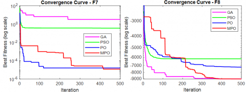
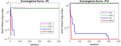
As Table 3 shows, the performance of MPO is always better than that of GA, PSO, and PO in the unimodal and simple multimodal functions (F1-F11). The algorithm of the MPO regularly delivers minimum, mean, and standard deviation values with nearly zero or zero error measurements, implying the extreme precision and stability of the algorithm. As an example in F1, MPO reached a lowest objective value of 0.00, and this is very good when compared with the results of GA (8.63E3) and the results of PSO (6.62E2). This demonstrates a better convergence behavior and an effective evasion of local optima on less complex problem landscapes than MPO has.
Table 3. Test results on CEC2017 (unimodal and simple multi-modal functions)
|
Function |
Criteria |
GA |
PSO |
PO |
MPO |
|
F1 |
std |
1.07E+03 |
2.18E+02 |
5.09E-38 |
0.00E+00 |
|
avg |
1.01E+04 |
9.10E+02 |
1.61E-38 |
0.00E+00 |
|
|
min |
8.63E+03 |
6.62E+02 |
2.20E-75 |
0.00E+00 |
|
|
F2 |
std |
2.44E+00 |
2.32E+00 |
5.73E-15 |
0.00E+00 |
|
avg |
3.18E+01 |
1.42E+01 |
1.88E-15 |
0.00E+00 |
|
|
min |
2.84E+01 |
1.19E+01 |
1.43E-43 |
0.00E+00 |
|
|
F3 |
std |
2.40E+03 |
7.75E+02 |
3.91E-31 |
0.00E+00 |
|
avg |
3.05E+04 |
3.03E+03 |
1.84E-31 |
0.00E+00 |
|
|
min |
1.66E+00 |
4.93E+00 |
1.44E-23 |
0.00E+00 |
|
|
F4 |
std |
5.36E+01 |
1.93E+01 |
6.33E-24 |
0.00E+00 |
|
avg |
5.16E+01 |
1.14E+01 |
1.29E-36 |
0.00E+00 |
|
|
min |
1.66E+00 |
4.93E+00 |
1.44E-23 |
0.00E+00 |
|
|
F5 |
std |
1.61E+06 |
4.67E+04 |
6.50E-04 |
1.17E+00 |
|
avg |
1.17E+07 |
9.11E+04 |
2.61E-04 |
1.90E+00 |
|
|
min |
9.11E+06 |
2.72E+04 |
2.08E-09 |
4.21E-01 |
|
|
F6 |
std |
1.49E+03 |
3.55E+02 |
2.66E-06 |
3.00E-02 |
|
avg |
9.15E+03 |
7.64E+02 |
1.55E-06 |
3.55E-02 |
|
|
min |
7.36E+03 |
4.28E+02 |
5.61E-13 |
4.85E-03 |
|
|
F7 |
std |
8.93E-01 |
1.39E-01 |
1.23E-05 |
1.01E-05 |
|
avg |
4.81E+00 |
2.36E-01 |
1.54E-05 |
9.16E-06 |
|
|
min |
3.28E+00 |
7.52E-02 |
1.04E-06 |
2.14E-06 |
|
|
F8 |
std |
3.81E+02 |
9.67E+02 |
1.18E+03 |
6.46E+02 |
|
avg |
-9.00E+03 |
-6.33E+03 |
-7.60E+03 |
-7.96E+03 |
|
|
min |
-9.77E+03 |
-7.53E+03 |
-1.02E+04 |
-9.41E+03 |
|
|
F9 |
std |
7.82E+00 |
1.75E+01 |
0.00E+00 |
0.00E+00 |
|
avg |
1.40E+02 |
7.97E+01 |
0.00E+00 |
0.00E+00 |
|
|
min |
1.26E+02 |
5.55E+01 |
0.00E+00 |
0.00E+00 |
|
|
F10 |
std |
4.42E-01 |
9.22E-01 |
0.00E+00 |
0.00E+00 |
|
avg |
1.50E+01 |
9.44E+00 |
8.88E-16 |
8.85E-16 |
|
|
min |
1.43E+01 |
8.25E+00 |
8.88E-16 |
8.75E-16 |
|
|
F11 |
std |
1.13E+01 |
4.45E+00 |
0.00E+00 |
0.00E+00 |
|
avg |
8.24E+01 |
9.36E+00 |
0.00E+00 |
0.00E+00 |
|
|
min |
6.36E+01 |
5.81E+00 |
0.00E+00 |
0.00E+00 |
3.2.2 Hybrid functions
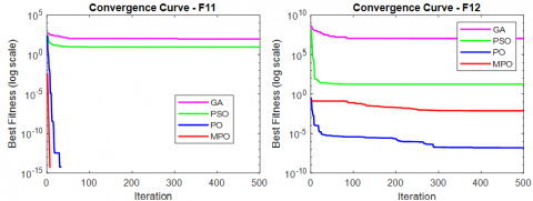
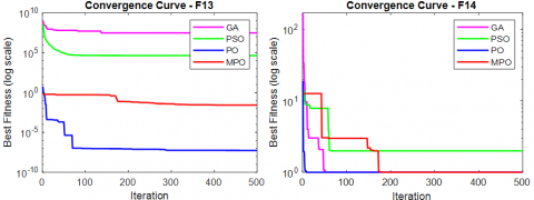
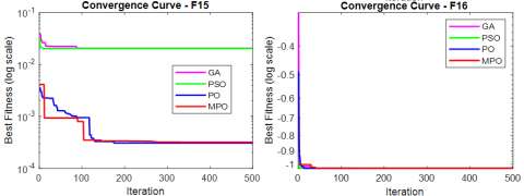
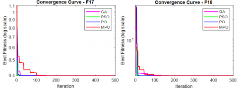
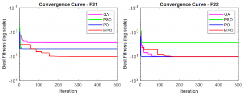
The results of the statistical analysis of the hybrid functions are given in Table 4. GA, PO algorithm, MPO, and PSO have some bad results on hybrid functions, but MPO is always better. In particular, in functions F12 to F21, MPO produces near-zero or zero error measures of minimum, mean, and standard deviation values. In line with that, in function F12, perfect performance was shown by MPO with 0.00 values in all metrics, which is inexplicably better than GA (6.36101) and PSO (5.81). The success of MPO in these functions indicates that MPO has a robust capability to converge as well as to avoid local minima. Algorithms such as the GA and PSO had shown large variance and worse performances in certain functions, whereas MPO repeated results many times and erred at a much lower percentage. Particularly, on functions F13, F14, F15, and others, MPO did not show frequent errors and had low values. In summary, the high accuracy of MPO on hybrid functions can be regarded as the strength of its local search ability and good ability to adapt to the complexity of the functions.
Table 4. Test results on CEC2017 (hybrid functions)
|
Function |
Criteria |
GA |
PSO |
PO |
MPO |
|
F12 |
std |
2.72E+06 |
6.57E+00 |
1.99E-07 |
1.83E-03 |
|
avg |
6.84E+06 |
1.38E+01 |
1.73E-07 |
2.20E-03 |
|
|
min |
1.75E+06 |
7.05E+00 |
3.40E-09 |
6.57E-04 |
|
|
F13 |
std |
1.04E+07 |
2.48E+04 |
5.82E-07 |
4.10E-02 |
|
avg |
3.39E+07 |
1.18E+04 |
3.75E-07 |
6.13E-02 |
|
|
min |
2.51E+07 |
1.35E+02 |
2.63E-10 |
1.86E-03 |
|
|
F14 |
std |
1.62E-06 |
3.26E+00 |
3.65E+00 |
6.42E-15 |
|
avg |
9.98E-01 |
3.36E+00 |
2.56E+00 |
9.98E-01 |
|
|
min |
9.98E-01 |
9.98E-01 |
9.98E-01 |
9.98E-01 |
|
|
F15 |
std |
8.41E-03 |
5.05E-04 |
4.71E-04 |
1.46E-04 |
|
avg |
5.90E-03 |
6.31E-04 |
6.76E-04 |
4.32E-04 |
|
|
min |
8.17E-04 |
3.07E-04 |
3.07E-04 |
3.10E-04 |
|
|
F16 |
std |
1.54E-04 |
0.00E+00 |
1.76E-11 |
1.95E-12 |
|
avg |
-1.03E+00 |
-1.03E+00 |
-1.03E+00 |
-1.03E+00 |
|
|
min |
-1.03E+00 |
-1.03E+00 |
-1.03E+00 |
-1.03E+00 |
|
|
F17 |
std |
1.23E-04 |
0.00E+00 |
6.20E-10 |
4.57E-12 |
|
avg |
3.98E-01 |
3.98E-01 |
3.98E-01 |
3.98E-01 |
|
|
min |
3.98E-01 |
3.98E-01 |
3.98E-01 |
3.98E-01 |
|
|
F18 |
std |
1.78E+00 |
1.48E-16 |
3.69E-09 |
1.02E-11 |
|
avg |
3.98E+00 |
3.00E+00 |
3.00E+00 |
3.00E+00 |
|
|
min |
3.00E+00 |
3.00E+00 |
3.00E+00 |
3.00E+00 |
|
|
F19 |
std |
1.04E-05 |
9.00E-16 |
9.62E-06 |
1.97E-07 |
|
avg |
-3.86E+00 |
-3.86E+00 |
-3.86E+00 |
-3.86E+00 |
|
|
min |
-3.86E+00 |
-3.86E+00 |
-3.86E+00 |
-3.86E+00 |
|
|
F20 |
std |
5.01E-02 |
5.74E-02 |
6.88E-02 |
8.08E-02 |
|
avg |
-3.30E+00 |
-3.29E+00 |
-3.29E+00 |
-3.26E+00 |
|
|
min |
-3.32E+00 |
-3.32E+00 |
-3.32E+00 |
-3.32E+00 |
|
|
F21 |
std |
-3.16E+00 |
-3.42E+00 |
2.46E+00 |
1.23E-05 |
|
avg |
-4.16E+00 |
-5.39E+00 |
-6.58E+00 |
-1.02E+01 |
|
|
min |
-1.02E+01 |
-1.02E+01 |
-1.02E+01 |
-1.02E+01 |
3.2.3 Composition and extended unimodal functions
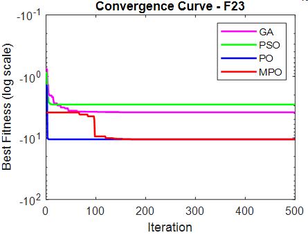
Table 5 will show the statistics of the composition and unimodal functions of the extended type. In the studied scenario, MPO dominates the rest of the four, such as GA, PSO, and PO, in both F22 and F23 functions. MPOs got the highest possible objective value of -1.04E+01 in every aspect, such as minimum, mean, and standard deviation, and the evidence of its excellence in precision and robustness compared to the other algorithms. In each case of F22 and F23, the optimum value of MPO retained its best value of -1.04E+01 across runs with a very low standard deviation (4.56E-05 for F22 and 8.67E-05 for F23); there were also big savings, surpassing 24. These values provide a greater degree of certainty as to the consistent outcome of MPO. This can be compared with GA, PSO, and PO, which had a bit bigger variance and a less steady output in various runs. It can be seen that MPO is exponentially convergent, that it does not get stuck in local minima, and that it performs very well in finding optimal or near-optimal solutions of composition and extended unimodal functions. The performance of MPO is especially outstanding due to its tendency to display high accuracy and low variation, unlike other algorithms used to carry out these kinds of functions, which makes it the most reliable algorithm. The outcomes of the t-test of the MPO values against the remainder of the algorithms still show Not a Number (NaN), even with the application of a small perturbation. This implies that the data would be similar to an extent of catastrophic cancellation/precision loss, thereby making the test render invaluable results. The value of the MPO is too small or near the range of the other algorithms; hence, the t-test does not give valid results. The non-parametric test option (e.g., the Mann-Whitney U test) would fit better in this case.
Table 5. Test results on CEC2017 (composition functions and extended unimodal functions)
|
Function |
Criteria |
GA |
PSO |
PO |
MPO |
|
F22 |
std |
3.83E+00 |
3.71E+00 |
2.80E+00 |
4.56E-05 |
|
avg |
-6.78E+00 |
-7.58E+00 |
-7.75E+00 |
-1.04E+01 |
|
|
min |
-1.04E+01 |
-1.04E+01 |
-1.04E+01 |
-1.04E+01 |
|
|
F23 |
std |
3.16E+00 |
3.42E+00 |
2.46E+00 |
1.23E-05 |
|
avg |
-4.16E+00 |
-5.39E+00 |
-6.58E+00 |
-1.02E+01 |
|
|
min |
-1.02E+01 |
-1.02E+01 |
-1.02E+01 |
-1.02E+01 |
Based on the results of the Mann-Whitney U test, the MPO algorithm does not perform significantly differently from the rest of the algorithms (GA, PSO, PO) on most comparisons. The majority of the p-values are based on a comparison of the functions F12-F22 = 1.0, which means that the difference between MPO and other algorithms is not insignificant. To illustrate this, one can use the F19 dataset and compare MPO with GA, in which case the p-value that will be shown is 1.0, indicating that the difference between the two algorithms cannot be considered to be significant. Likewise, when comparing MPO and PO in the case of F21, we ended up with a p-value of 0.5, which gives us the answer that the difference in the variation is not significant, but it is still higher than the threshold of 0.05, indicating that the difference was by chance. As a final conclusion of the tests, the statistical significance between MPO and the other algorithms is generally not different, and it is probable that the difference that is observed in performance is merely random. This is an indication that the high performance of MPO compared to the other algorithms could be what has been considered as a difference in algorithm and not the randomness or individual characteristics of the problem. According to the information provided in Table 5, which gives the results of the statistical test of the F22 and F23 functions of composition and extended unimodal functions, the t-test and the Mann-Whitney U test results indicate that the U-statistic becomes 0.0 and the corresponding p-value also becomes 1.0 where a comparison is attempted between the MPO algorithm and the other algorithms (GA, PSO, and PO) in the context of these two functions. The above outcome shows that there is no significant difference between the performance of MPO relative to the rest of the algorithms. A p-value of 1.0 indicates that whatever differences we see between the performance of the algorithms are probably not significant, which is to say not real or intrinsic, but rather due to chance variance.
In conclusion, based on the analysis of the composition and extended unimodal functions (F22 and F23) in Table 5, it can be concluded that the performance differences between MPO and the other algorithms (GA, PSO, and PO) are not statistically significant. This indicates that MPO's performance advantage does not represent a meaningful or reliable improvement over the other algorithms in these specific functions.
This paper uses different optimization algorithms that are applied to find the optimal switching angles of SHE and tuning the PWM parameters to a minimal harmonic distortion and producing high-quality smooth waveforms. Optimization algorithms used in this analysis are DE, NR, PSO, GA, PO, and MPO. DE and NR have the most effectiveness in the case of solution refinement. DE is an evolutionary optimization mechanism that is easily applied where a problem solution requires fine adjustments with dependencies among variables being highly complicated and non-linear. On the contrary, NR is a derivative-based optimization technique, which has a fast convergence speed and high accuracy in determining optimal solutions; this last feature is particularly useful in tasks that demand extreme accuracy. Globally, better search capability by PSO and GA is well known, and it does not fall in local minima and is therefore able to optimize SHE and PWM very well. PO and MPO, which offer improved exploration and exploitation capabilities, are especially useful in solving high-dimensional optimization problems that are comprised of complex constraints, which is the case of SHE and PWM optimization. The difference in the performances of the algorithms will also be associated with random variation and not the true performance difference. Tables 6 to 11 show the switching angles calculated using NR, DE, GA, PSO, PO, and MPO algorithms against the modulation index. In Table 6, the NR algorithm did not produce valid values for any modulation index. The best performance of the NR algorithm was observed in the modulation index range of 0.6 to 1.0. In contrast, the other algorithms (DE, GA, PSO, PO, and MPO) provided valid solutions in the modulation index range of 0.1 to 1.0.
Table 6. Calculated switching angles with NR versus modulation index
|
M |
Switching Angle (°) |
|
||||
|
θ1 |
θ2 |
θ3 |
θ4 |
θ5 |
Fitness |
|
|
0.1 |
NaN |
NaN |
NaN |
NaN |
NaN |
NaN |
|
0.2 |
NaN |
NaN |
NaN |
NaN |
NaN |
NaN |
|
0.3 |
NaN |
NaN |
NaN |
NaN |
NaN |
NaN |
|
0.4 |
NaN |
NaN |
NaN |
NaN |
NaN |
NaN |
|
0.5 |
NaN |
NaN |
NaN |
NaN |
NaN |
NaN |
|
0.6 |
35.34241 |
46.95268 |
58.57986 |
72.61202 |
87.83723 |
7.70E-08 |
|
0.7 |
3.58075 |
38.72273 |
40.59147 |
79.59416 |
88.24212 |
3.16E-08 |
|
0.8 |
22.34200 |
39.27860 |
52.68666 |
59.31913 |
70.96458 |
2.35E-08 |
|
0.9 |
7.65923 |
27.57052 |
40.78902 |
52.55991 |
73.03902 |
3.20E-08 |
|
1.0 |
7.85969 |
19.37252 |
29.65226 |
47.67984 |
63.21208 |
3.94E-08 |
Table 7. Calculated switching angles with DE versus modulation index
|
M |
Switching Angle (°) |
|
||||
|
θ1 |
θ2 |
θ3 |
θ4 |
θ5 |
Fitness |
|
|
0.1 |
66.87745 |
90.00000 |
90.00000 |
90.00000 |
90.00000 |
6.80E+01 |
|
0.2 |
43.40294 |
86.62569 |
90.00000 |
90.00000 |
90.00000 |
2.99E+01 |
|
0.3 |
44.37724 |
64.93482 |
89.24181 |
89.24181 |
89.24181 |
1.31E+01 |
|
0.4 |
39.06932 |
56.37971 |
76.07061 |
90.00000 |
90.00000 |
3.24E+00 |
|
0.5 |
36.71073 |
49.63060 |
65.51395 |
84.28121 |
89.99996 |
5.90E-01 |
|
0.6 |
35.34639 |
46.95243 |
58.58000 |
72.61352 |
87.83390 |
2.55E-05 |
|
0.7 |
3.54680 |
19.61564 |
38.92930 |
88.53521 |
89.69297 |
1.87E-04 |
|
0.8 |
9.70600 |
33.43350 |
43.30186 |
61.18042 |
83.59375 |
3.23E-04 |
|
0.9 |
7.67237 |
27.57788 |
40.80034 |
52.56281 |
73.02352 |
6.35E-04 |
|
1.0 |
7.85728 |
19.37792 |
29.64313 |
47.67738 |
63.21774 |
4.97E-05 |
Table 8. Calculated switching angles with GA versus modulation index
|
M |
Switching Angle (°) |
|
||||
|
θ1 |
θ2 |
θ3 |
θ4 |
θ5 |
Fitness |
|
|
0.1 |
73.59140 |
86.53116 |
88.77507 |
88.94033 |
89.42759 |
2.45E+02 |
|
0.2 |
56.43097 |
83.69524 |
85.51045 |
87.79158 |
89.66544 |
2.83E+02 |
|
0.3 |
39.15064 |
69.98930 |
88.46293 |
89.00127 |
89.08365 |
4.96E+01 |
|
0.4 |
48.69936 |
52.69994 |
75.00058 |
87.76345 |
89.56451 |
1.38E+02 |
|
0.5 |
30.73403 |
43.28971 |
73.18132 |
85.88549 |
89.26121 |
1.35E+02 |
|
0.6 |
35.36076 |
47.04300 |
58.68608 |
72.87854 |
87.86143 |
3.39E-01 |
|
0.7 |
34.20937 |
44.83793 |
53.81111 |
65.79321 |
77.73272 |
1.26E-01 |
|
0.8 |
9.72985 |
32.98099 |
43.29371 |
61.21547 |
83.90587 |
1.46E-01 |
|
0.9 |
15.68887 |
26.03203 |
45.14029 |
59.68781 |
62.45776 |
1.18E+00 |
|
1.0 |
8.21512 |
19.68559 |
30.03778 |
48.66304 |
63.52940 |
1.08E+00 |
Table 9. Calculated switching angles with PSO versus modulation index
|
M |
Switching Angle (°) |
|
||||
|
θ1 |
θ2 |
θ3 |
θ4 |
θ5 |
Fitness |
|
|
0.1 |
66.95172 |
89.93190 |
89.99989 |
89.99989 |
90.00000 |
6.87E+01 |
|
0.2 |
43.36757 |
86.89266 |
89.87690 |
89.88086 |
90.00000 |
3.00E+01 |
|
0.3 |
45.17798 |
65.48881 |
86.65664 |
90.00000 |
90.00000 |
1.69E+01 |
|
0.4 |
38.66593 |
59.51616 |
81.87406 |
81.87407 |
90.00000 |
1.16E+02 |
|
0.5 |
25.17878 |
49.37123 |
66.22901 |
89.75515 |
90.00000 |
3.94E+00 |
|
0.6 |
12.67486 |
35.09679 |
58.33990 |
87.85075 |
90.00000 |
3.26E-01 |
|
0.7 |
35.20547 |
44.29895 |
54.16490 |
65.07726 |
77.92172 |
6.52E-01 |
|
0.8 |
9.70003 |
33.43707 |
43.29479 |
61.18008 |
83.59806 |
3.49E-01 |
|
0.9 |
16.27231 |
25.95065 |
44.80686 |
61.12850 |
61.12853 |
3.64E-01 |
|
1.0 |
7.77741 |
19.44091 |
29.46680 |
47.61562 |
63.35493 |
3.53E-02 |
Table 10. Calculated switching angles with PO versus modulation index
|
M |
Switching Angle (°) |
|
||||
|
θ1 |
θ2 |
θ3 |
θ4 |
θ5 |
Fitness |
|
|
0.1 |
66.52601 |
90.00000 |
90.00000 |
90.00000 |
90.00000 |
1.49E+01 |
|
0.2 |
39.95489 |
88.91996 |
90.00000 |
90.00000 |
90.00000 |
4.61E+01 |
|
0.3 |
43.41066 |
64.70951 |
88.59417 |
90.00000 |
90.00000 |
2.78E+01 |
|
0.4 |
38.53115 |
55.23116 |
77.39299 |
90.00000 |
90.00000 |
6.95E+00 |
|
0.5 |
23.79056 |
49.72707 |
65.68991 |
90.00000 |
90.00000 |
1.83E+00 |
|
0.6 |
35.34241 |
46.95278 |
58.57993 |
72.61213 |
87.83734 |
2.65E-11 |
|
0.7 |
3.58063 |
38.72337 |
40.59086 |
79.59423 |
88.24206 |
3.31E-09 |
|
0.8 |
9.31145 |
25.40075 |
42.39083 |
61.36071 |
88.07622 |
8.51E-03 |
|
0.9 |
7.61467 |
27.48060 |
40.92180 |
52.64664 |
72.92235 |
4.34E-02 |
|
1.0 |
7.85978 |
19.37250 |
29.65223 |
47.67999 |
63.21216 |
8.24E-04 |
Table 11. Calculated switching angles with MPO versus modulation index
|
M |
Switching Angle (°) |
|
||||
|
θ1 |
θ2 |
θ3 |
θ4 |
θ5 |
Fitness |
|
|
0.1 |
66.87745 |
90.00000 |
90.00000 |
90.00000 |
90.00000 |
6.79E+01 |
|
0.2 |
43.34711 |
86.66410 |
90.00000 |
90.00000 |
90.00000 |
2.99E+01 |
|
0.3 |
44.56114 |
64.68998 |
88.19084 |
89.62763 |
89.99945 |
1.33E+01 |
|
0.4 |
39.06837 |
56.39925 |
76.05447 |
90.00000 |
90.00000 |
3.24E+00 |
|
0.5 |
36.71314 |
49.63082 |
65.51593 |
84.27774 |
90.00000 |
5.97E-01 |
|
0.6 |
35.34205 |
46.95254 |
58.58022 |
72.61191 |
87.83768 |
7.00E-07 |
|
0.7 |
19.62499 |
38.94352 |
56.46641 |
63.54021 |
88.21087 |
8.91E-06 |
|
0.8 |
22.26677 |
39.18881 |
52.68885 |
59.27126 |
70.93771 |
3.14E-07 |
|
0.9 |
7.66560 |
27.56387 |
40.77631 |
52.57904 |
73.03351 |
8.37E-04 |
|
1.0 |
7.86377 |
19.39269 |
29.63815 |
47.68469 |
63.20828 |
7.49E-30 |
Based on the data from Tables 12 to 17, the switching angles and THD minimization performance of different algorithms (NR, DE, GA, PSO, PO, and MPO) are compared against modulation indices. The NR algorithm failed to provide valid results for low modulation indices (M = 0.1, 0.2, 0.3, 0.4), often yielding "NaN" values. However, from M = 0.6 onwards, NR provided valid results, showing the best performance between modulation indices of 0.6 and 1.0. Other algorithms (DE, GA, PSO, PO, MPO) were able to offer a broader solution range across the 0.1 to 1.0 modulation index range. The DE algorithm was particularly effective at low and medium modulation indices, while the GA algorithm performed better at higher modulation indices. The PSO algorithm showed success in lower modulation index ranges, whereas the PO algorithm generally provided more stable results. The MPO algorithm delivered high accuracy across all modulation indices but showed some anomalies at M = 0.9. In conclusion, each algorithm exhibited different performances at specific modulation indices; the choice of the most suitable algorithm depends on the system's requirements.
Table 12. NR algorithm for switching angles and THD minimization at various modulation indices
|
M |
Vref (rms) |
V1p (rms) |
Error (%) |
THD (%) |
THDE (%) |
h5 |
h7 |
h11 |
h13 |
|
0.1 |
Na N |
Na N |
Na N |
Na N |
Na N |
Na N |
Na N |
Na N |
Na N |
|
0.2 |
Na N |
Na N |
Na N |
Na N |
Na N |
Na N |
Na N |
Na N |
Na N |
|
0.3 |
Na N |
Na N |
Na N |
Na N |
Na N |
Na N |
Na N |
Na N |
Na N |
|
0.4 |
Na N |
Na N |
Na N |
Na N |
Na N |
Na N |
Na N |
Na N |
Na N |
|
0.5 |
Na N |
Na N |
Na N |
Na N |
Na N |
Na N |
Na N |
Na N |
Na N |
|
0.6 |
63.64 |
63.44 |
3.14E-03 |
6.84 |
0.04 |
0.01 |
0.01 |
0.02 |
0.02 |
|
0.7 |
74.25 |
73.96 |
3.91E-03 |
7.92 |
0.08 |
0.02 |
0.05 |
0.04 |
0.02 |
|
0.8 |
84.85 |
84.5 |
4.12E-03 |
6.72 |
0.03 |
0.01 |
0.02 |
0.01 |
0.01 |
|
0.9 |
95.46 |
95.08 |
3.98E-03 |
6.34 |
0.04 |
0.02 |
0.03 |
0.01 |
0.03 |
|
1.0 |
106.07 |
105.6 |
4.43E-03 |
5.03 |
0.04 |
0.01 |
0.01 |
0.03 |
0.02 |
Table 13. DE algorithm for switching angles and THD minimization at various modulation indices
|
M |
VREF (rms) |
V1p (rms) |
Error (%) |
THD (%) |
THDE (%) |
h5 |
h7 |
h11 |
h13 |
|
0.1 |
10.61 |
10.59 |
1.89E-03 |
59.38 |
55.11 |
46.64 |
11.71 |
21.98 |
10.70 |
|
0.2 |
21.21 |
21.19 |
9.43E-04 |
27.95 |
18.18 |
12.72 |
2.68 |
12.56 |
1.98 |
|
0.3 |
31.82 |
31.72 |
3.14E-03 |
21.10 |
8.09 |
4.68 |
3.60 |
0.48 |
5.51 |
|
0.4 |
42.43 |
42.30 |
3.06E-03 |
12.84 |
3.15 |
2.37 |
1.06 |
1.69 |
0.57 |
|
0.5 |
53.03 |
52.87 |
3.02E-03 |
9.07 |
1.09 |
0.47 |
0.34 |
0.81 |
0.44 |
|
0.6 |
63.64 |
63.44 |
3.14E-03 |
6.84 |
0.04 |
0.01 |
0.01 |
0.02 |
0.02 |
|
0.7 |
74.25 |
73.97 |
3.77E-03 |
8.21 |
0.03 |
0.02 |
0.01 |
0.00 |
0.01 |
|
0.8 |
84.85 |
84.53 |
3.77E-03 |
5.64 |
0.04 |
0.00 |
0.03 |
0.01 |
0.01 |
|
0.9 |
95.46 |
95.05 |
4.29E-03 |
6.34 |
0.04 |
0.00 |
0.03 |
0.01 |
0.00 |
|
1.0 |
106.07 |
105.6 |
4.43E-03 |
5.03 |
0.04 |
0.01 |
0.01 |
0.03 |
0.02 |
Table 14. GA algorithm for switching angles and THD minimization at various modulation indices
|
M |
VREF (rms) |
V1p (rms) |
Error (%) |
THD (%) |
THDE (%) |
h5 |
h7 |
h11 |
h13 |
|
0.1 |
10.61 |
10.57 |
3.77E-03 |
123.90 |
103.96 |
78.46 |
60.74 |
26.81 |
15.55 |
|
0.2 |
21.21 |
21.14 |
3.30E-03 |
64.86 |
56.18 |
34.17 |
12.91 |
26.96 |
33.10 |
|
0.3 |
31.82 |
31.74 |
2.51E-03 |
25.45 |
15.18 |
5.62 |
12.06 |
2.38 |
6.92 |
|
0.4 |
42.43 |
42.27 |
3.77E-03 |
21.87 |
18.73 |
8.14 |
5.92 |
14.65 |
5.89 |
|
0.5 |
53.03 |
52.79 |
4.53E-03 |
16.62 |
13.10 |
3.00 |
12.66 |
1.27 |
0.76 |
|
0.6 |
63.64 |
63.27 |
5.81E-03 |
6.78 |
0.22 |
0.10 |
0.12 |
0.10 |
0.11 |
|
0.7 |
74.25 |
73.93 |
4.31E-03 |
5.60 |
0.35 |
0.09 |
0.19 |
0.19 |
0.21 |
|
0.8 |
84.85 |
84.46 |
4.60E-03 |
5.80 |
0.23 |
0.09 |
0.10 |
0.09 |
0.16 |
|
0.9 |
95.46 |
95.07 |
4.09E-03 |
6.37 |
0.73 |
0.01 |
0.54 |
0.39 |
0.29 |
|
1.0 |
106.07 |
105.00 |
1.01E-02 |
5.31 |
0.28 |
0.15 |
0.11 |
0.02 |
0.21 |
Table 15. PSO algorithm for switching angles and THD minimization at various modulation indices
|
M |
VREF (rms) |
V1p (rms) |
Error (%) |
THD (%) |
THDE (%) |
h5 |
h7 |
h11 |
h13 |
|
0.1 |
10.61 |
10.61 |
0.00E+00 |
59.50 |
55.21 |
46.50 |
12.09 |
21.65 |
16.47 |
|
0.2 |
21.21 |
21.16 |
2.36E-03 |
28.75 |
18.27 |
13.02 |
2.76 |
12.33 |
2.12 |
|
0.3 |
31.82 |
31.74 |
2.51E-03 |
20.47 |
9.16 |
7.44 |
2.10 |
2.54 |
4.19 |
|
0.4 |
42.43 |
42.28 |
3.54E-03 |
21.18 |
17.97 |
10.08 |
10.18 |
6.72 |
8.50 |
|
0.5 |
53.03 |
52.86 |
3.21E-03 |
9.52 |
2.66 |
0.86 |
2.15 |
0.27 |
1.27 |
|
0.6 |
63.64 |
63.41 |
3.61E-03 |
6.87 |
0.63 |
0.07 |
0.09 |
0.19 |
0.55 |
|
0.7 |
74.25 |
73.97 |
3.77E-03 |
5.99 |
0.79 |
0.29 |
0.51 |
0.06 |
0.53 |
|
0.8 |
84.85 |
84.53 |
3.77E-03 |
5.81 |
0.23 |
0.06 |
0.13 |
0.06 |
0.15 |
|
0.9 |
95.46 |
95.07 |
4.09E-03 |
7.12 |
0.47 |
0.25 |
0.15 |
0.14 |
0.33 |
|
1.0 |
106.07 |
105.6 |
4.43E-03 |
5.02 |
0.12 |
0.05 |
0.10 |
0.05 |
0.03 |
Table 16. PO algorithm for switching angles and THD minimization at various modulation indices
|
M |
VREF (rms) |
V1p (rms) |
Error (%) |
THD (%) |
THDE (%) |
h5 |
h7 |
h11 |
h13 |
|
0.1 |
10.61 |
10.72 |
-1.04E-02 |
57.75 |
53.38 |
44.72 |
9.79 |
22.36 |
15.91 |
|
0.2 |
21.21 |
21.17 |
1.89E-03 |
27.03 |
22.57 |
21.54 |
0.55 |
0.28 |
6.73 |
|
0.3 |
31.82 |
31.72 |
3.14E-03 |
18.19 |
8.85 |
2.13 |
4.14 |
1.98 |
7.27 |
|
0.4 |
42.43 |
42.29 |
3.30E-03 |
12.82 |
4.37 |
0.30 |
0.99 |
3.48 |
2.43 |
|
0.5 |
53.03 |
53.1 |
1.63E-01 |
6.89 |
1.61 |
0.01 |
1.19 |
0.65 |
0.87 |
|
0.6 |
63.64 |
63.31 |
5.19E-03 |
6.84 |
0.04 |
0.01 |
0.01 |
0.02 |
0.02 |
|
0.7 |
74.25 |
73.92 |
4.44E-03 |
7.92 |
0.08 |
0.02 |
0.05 |
0.04 |
0.02 |
|
0.8 |
84.85 |
84.52 |
3.89E-03 |
6.80 |
0.08 |
0.04 |
0.05 |
0.01 |
0.03 |
|
0.9 |
95.46 |
134.5 |
-4.09E-01 |
6.31 |
0.15 |
0.10 |
0.10 |
0.01 |
0.02 |
|
1.0 |
106.07 |
105.6 |
4.43E-03 |
5.03 |
0.04 |
0.01 |
0.01 |
0.03 |
0.02 |
Table 17. MPO algorithm for switching angles and THD minimization at various modulation indices
|
M |
VREF (rms) |
V1p (rms) |
Error (%) |
THD (%) |
THDE (%) |
h5 |
h7 |
h11 |
h13 |
|
0.1 |
10.61 |
10.57 |
3.77E-03 |
59.35 |
55.17 |
46.09 |
11.48 |
22.31 |
17.01 |
|
0.2 |
21.21 |
21.16 |
2.36E-03 |
27.64 |
18.16 |
13.13 |
2.72 |
12.19 |
2.19 |
|
0.3 |
31.82 |
31.75 |
2.20E-03 |
20.06 |
8.08 |
4.52 |
4.24 |
0.65 |
5.15 |
|
0.4 |
42.43 |
42.27 |
3.77E-03 |
12.86 |
3.03 |
2.30 |
0.99 |
1.62 |
0.50 |
|
0.5 |
53.03 |
52.86 |
3.21E-03 |
9.04 |
1.06 |
0.50 |
0.31 |
0.79 |
0.41 |
|
0.6 |
63.64 |
63.44 |
3.14E-03 |
6.84 |
0.04 |
0.01 |
0.01 |
0.02 |
0.02 |
|
0.7 |
74.25 |
73.98 |
3.64E-03 |
5.56 |
0.05 |
0.02 |
0.02 |
0.03 |
0.01 |
|
0.8 |
84.85 |
84.53 |
3.77E-03 |
5.64 |
0.04 |
0.00 |
0.03 |
0.01 |
0.01 |
|
0.9 |
95.46 |
95.07 |
4.09E-03 |
6.34 |
0.05 |
0.02 |
1.00 |
0.01 |
0.01 |
|
1.0 |
106.07 |
105.6 |
4.43E-03 |
5.02 |
0.04 |
0.02 |
0.02 |
0.01 |
0.01 |
Figure 3. Convergence curves of the proposed and compared functions on CEC2017
Figure 3 illustrates the convergence curves of the proposed and compared functions on CEC2017, highlighting the relative performance of each function in terms of convergence speed and stability. The GA, PSO, PO, and MPO algorithms were compared in this context.
Table 18 presents the switching angles and corresponding fitness function values calculated by all algorithms for a given modulation index. As observed, the MPO algorithm achieved the best performance, delivering the lowest fitness value. The PO algorithm followed closely, achieving the second-best performance. In contrast, the GA algorithm yielded the least favorable results, demonstrating the highest fitness value among the tested algorithms. This analysis indicates that MPO is the most effective algorithm for minimizing the fitness function, while PO also performs well. On the other hand, GA exhibits less efficiency in comparison to the other methods tested.
Table 18. Algorithm results for modulation index = 1
|
Algorithm |
Switching Angle (°) |
|
||||
|
θ1 |
θ2 |
θ3 |
θ4 |
θ5 |
Fitness |
|
|
NR |
7.85969 |
19.37252 |
29.65226 |
47.67984 |
63.21208 |
3.94E-08 |
|
DE |
7.85728 |
19.37792 |
29.64313 |
47.67738 |
63.21774 |
4.97E-05 |
|
GA |
8.21512 |
19.68559 |
30.03778 |
48.66304 |
63.52940 |
1.08E+00 |
|
PSO |
7.77741 |
19.44091 |
29.46680 |
47.61562 |
63.35493 |
3.53E-02 |
|
PO |
7.85978 |
19.37250 |
29.65223 |
47.67999 |
63.21216 |
8.24E-04 |
|
MPO |
7.86377 |
19.39269 |
29.63815 |
47.68469 |
63.20828 |
7.49E-30 |
Table 19. Simulation results for switching angles and THD minimization at various modulation indices using different algorithms (for M=1.0)
|
Algorithm |
V1p (rms) |
Error (%) |
THD (%) |
THDe (%) |
h5 |
h7 |
h11 |
h13 |
|
NR |
105.6 |
4.43E-03 |
5.03 |
0.04 |
0.01 |
0.01 |
0.03 |
0.02 |
|
DE |
105.6 |
4.43E-03 |
5.03 |
0.04 |
0.01 |
0.01 |
0.03 |
0.02 |
|
GA |
105.0 |
1.01E-02 |
5.31 |
0.28 |
0.15 |
0.11 |
0.02 |
0.21 |
|
PSO |
105.6 |
4.43E-03 |
5.02 |
0.12 |
0.05 |
0.10 |
0.05 |
0.03 |
|
PO |
105.6 |
4.43E-03 |
5.03 |
0.04 |
0.01 |
0.01 |
0.03 |
0.02 |
|
MPO |
105.6 |
4.43E-03 |
5.02 |
0.04 |
0.02 |
0.02 |
0.01 |
0.01 |
The values provided in Table 18 have been applied to the inverter in the MATLAB Simulink environment, and the simulation results are presented in Table 19.
In Table 19, the performance of different optimization algorithms—NR, DE, GA, PSO, PO, and MPO—is compared in terms of several key metrics: V1p(rms), error percentage, THD, THDe, and the contributions of specific harmonics (h5, h7, h11, h13).
Based on the results, the NR, DE, PO, and MPO algorithms perform similarly in terms of output voltage, error, THD, and harmonic components. GA shows a slightly higher error and THD, suggesting it performs less efficiently than the other algorithms in minimizing these parameters. However, all algorithms exhibit reasonable results, with MPO being particularly effective in minimizing harmonic distortion while maintaining satisfactory performance across all parameters.
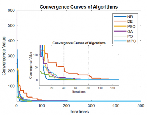
Figure 4. Convergence graph for a modulation index of 1
Based on the convergence curves in Figure 4, we can observe that MPO and PO exhibit the fastest convergence, reaching near-zero values in fewer iterations, indicating their efficiency in quickly finding optimal or near-optimal solutions. Conversely, NR exhibits a more non-linear decline, hence taking an extended period to reach smaller convergence values, and this implies that it can be slower in arriving at an optimal solution. Although it is effective, DE and GA show slower convergence than MPO and PO and display observable fluctuations in each iteration. The convergent speed of PSO is slow compared to MPO and PO, though it will finally arrive at a similar outcome. The numbers indicate that MPO and PO are most appropriate to those problems where high-speed convergence is more relevant, and at the same time, DE, GA, and PSO might be preferred to those optimization problems that have a complex solution space and where it may be necessary to look further in the solution space. In general, MPO and PO provide highly efficient and faster convergence, so they are most suitable when it comes to time-critical optimization objectives. Table 20 contains the details about the number of functions called and the computation times of the diverse optimization algorithms (NR, DE, GA, PSO, PO, and MPO), five times with M=1.0. NR supports the least number of functions with an average of 3.60E-04; however, it can only be applied in a very specific manner. DE and GA involve more calls to functions with means of 1.78E-01 and 2.24E-01, respectively, and these values are more spread across runs. PSO is more efficient with function calls, with the mean being 4.99E-02, followed by PO, which also seems to be very much comparable to PSO, with a mean of 3.97E-02. MPO uses 1.58E-01 calls to functions, and in its performance, it is steady but not very efficient compared to PSO and PO. Generally, PSO and PO present the optimal level of stability and efficiency to carry out real-time tasks in optimization.
Table 20. The number of function calls to reach the optimum value and computation time (for M=1.0)
|
Algorithm |
Run Number |
AVG |
||||
|
1 |
2 |
3 |
4 |
5 |
||
|
NR |
1.00E-04 |
7.00E-04 |
7.00E-04 |
1.00E-04 |
2.00E-04 |
3.60E-04 |
|
DE |
1.84E-01 |
1.63E-01 |
1.70E-01 |
1.74E-01 |
1.97E-01 |
1.78E-01 |
|
GA |
1.81E-01 |
2.13E-01 |
2.53E-01 |
2.30E-01 |
2.42E-01 |
2.24E-01 |
|
PSO |
7.54E-02 |
5.18E-02 |
3.93E-02 |
4.43E-02 |
3.89E-02 |
4.99E-02 |
|
PO |
4.76E-02 |
4.10E-02 |
3.71E-02 |
2.58E-02 |
4.69E-02 |
3.97E-02 |
|
MPO |
2.01E-01 |
1.52E-01 |
1.57E-01 |
1.27E-01 |
1.55E-01 |
1.58E-01 |
In this study, the performance of various optimization algorithms—NR, DE, GA, PSO, PO, and MPO—was evaluated for switching angle calculation and THD minimization at different modulation indices. The results, as presented in Tables 8-13, indicate notable differences in the performance of these algorithms. NR failed to deliver valid results for lower modulation indices (M = 0.1, 0.2, 0.3, and 0.4), with "NaN" values observed, but performed reasonably well between M = 0.6 and M = 1.0. In contrast, other algorithms, such as DE, GA, PSO, PO, and MPO, provided valid results across the entire range of modulation indices (M = 0.1 to 1.0). While DE and PSO excelled at lower modulation indices, GA performed best at higher M values. PO and MPO provided stable and reliable results across all modulation indices.
Subsequent critique, especially on Table 19, showed that MPO was the best-performing algorithm with regard to both the calculation of the switching angle and the reduction of THD, as well as having the smallest THD value and being close to the correct value calculation results in switching angles. Comparatively, the lowest performance was seen in GA, which recorded maximum errors and THD, especially at lower modulation indices. The harmonic contributions were also minimal in all indices of modulation in the case of MPO, meaning that the harmonic deviation was less when compared to GA, which also presented large harmonic deviations. The main value added of this research is the illustration of how the optimization algorithm that would suit SwA calculation and THD minimization is the MPO. It is also able to produce the lowest THD and the best switching angle precision. The resilient and consistent performance of MPO with iterations of modulation indices under consideration does not report failure even in some other algorithms, especially GA, hence becoming the most optimal algorithm to apply in switching angle computation and minimizing THD. The outstanding performance received by MPO is explained by the special structure and built-in characteristics. In contrast to classical optimization approaches, MPO includes a strong search scheme that is able to respond to the problem space effectively. It converges with fewer steps and correctly in high-dimensional/difficult tasks because it does not get caught up in local minima. MPO shows stable convergence properties through all modulation indices and is extremely convenient in situations with complex optimization because, as is the case with THD, the solution space is nonlinear and multimodal.
The feasibility of the inverter design is very important in real-time applications, as minimizing THD and the exact determination of switching angles are essential. The capability of MPO to reduce THD and precisely calculate switching angles would increase the efficiency and reliability of inverter systems. A low THD culminates in better power quality and minimized system losses, leading to optimal performance of the system. Also, the modulation flexibility of MPO is suitable in many operating scenarios, as it can be utilized under diverse modulation indices. MPO incorporated in real-time or embedded inverter systems can add tremendously high levels of performance to the reliability of such systems so that power converters perform to their best. To apply to such systems, MPO can be optimized further to decrease the time of calculations. To improve the real-time performance of MPO, hardware accelerators such as an FPGA or GPU may be used. The next step is to look at hybrid models that would hybridize MPO and machine learning algorithms in order to predict switching angles dynamically, depending on the operating conditions, in order to augment the performance of inverter systems in industrial settings.
[1] Al-Khaled, K., Taha, S.N. (2022). Efficient solutions for nonlinear diffusion equations appeared as models of physical problems. Mathematical Modelling of Engineering Problems, 9(6): 1508-1514. https://doi.org/10.18280/mmep.090610
[2] Phoosree, S., Suphattanakul, O., Maliwan, E., Senmoh, M., et al. (2023). Novel solutions to fractional nonlinear equations for crystal dislocation and ocean shelf internal waves via the generalized Bernoulli equation method. Mathematical Modelling of Engineering Problems, 10(3): 821-828. https://doi.org/10.18280/mmep.100312
[3] Alzaareer, K., Salem, Q., El-Bayeh, C.Z., Harasis, S., et al. (2022). Development of new admittance matrix for newton-Raphson power flow in distribution networks. Mathematical Modelling of Engineering Problems, 9(1): 168-177. https://doi.org/10.18280/mmep.090121
[4] Karaca, H., Bektas, E. (2015). Selective harmonic elimination technique based on genetic algorithm for multilevel inverters. In The World Congress on Engineering and Computer Science, Springer, Singapore, pp. 333-347. https://doi.org/10.1007/978-981-10-2717-8_24
[5] Zeng, T., Wang, W., Wang, H., Cui, Z., et al. (2022). Artificial bee colony based on adaptive search strategy and random grouping mechanism. Expert Systems with Applications, 192: 116332. https://doi.org/10.1016/j.eswa.2021.116332
[6] Wang, S., Li, Y., Yang, H., Liu, H. (2018). Self-adaptive differential evolution algorithm with improved mutation strategy. Soft Computing, 22(11): 3433-3447. https://doi.org/10.1007/s00500-017-2588-5
[7] Iqbal, I., Boulaaras, S.M., Althobaiti, S., Althobaiti, A., et al. (2025). Exploring soliton dynamics in the nonlinear Helmholtz equation: Bifurcation, chaotic behavior, multistability, and sensitivity analysis. Nonlinear Dynamics, 113(13): 16933-16954. https://doi.org/10.1007/s11071-025-10961-3
[8] ur Rahman, M., Sun, M., Boulaaras, S., Baleanu, D. (2024). Bifurcations, chaotic behavior, sensitivity analysis, and various soliton solutions for the extended nonlinear Schrödinger equation. Boundary Value Problems, 2024(1): 15. https://doi.org/10.1186/s13661-024-01825-7
[9] Casella, F., Bachmann, B. (2021). On the choice of initial guesses for the Newton-Raphson algorithm. Applied Mathematics and Computation, 398: 125991. https://doi.org/10.1016/j.amc.2021.125991
[10] Sienicki, K. (2024). Comment on the paper titled ‘the origin of quantum mechanical statistics: Insights from research on human language’ (arXiv preprint arXiv: 2407.14924, 2024). Preprints.org. https://doi.org/10.20944/preprints202411.2377.v1
[11] Mousavirad, S.J., Schaefer, G., Korovin, I., Moghadam, M.H., et al. (2021). An enhanced differential evolution algorithm using a novel clustering-based mutation operator. In 2021 IEEE International Conference on Systems, Man, and Cybernetics (SMC), Melbourne, Australia, pp. 176-181. https://doi.org/10.1109/smc52423.2021.9658743
[12] Taha, T.A., Shalaby, M., Wahab, N.I.A., Zaynal, H.I., et al. (2025). Recent advancements in multilevel inverters: Topologies, modulation techniques, and emerging applications. Symmetry, 17(7): 1010. https://doi.org/10.3390/sym17071010
[13] Pourdadashnia, A., Farhadi-Kangarlu, M., Sadoughi, M. (2021). Staircase selective harmonic elimination in multilevel inverters to achieve wide output voltage range. In 2021 12th Power Electronics, Drive Systems, and Technologies Conference (PEDSTC), Tabriz, Iran, pp. 1-6. https://doi.org/10.1109/pedstc52094.2021.9405826
[14] Ceylan, O., Neshat, M., Mirjalili, S. (2024). Cascaded H-bridge multilevel inverters optimization using adaptive grey wolf optimizer with local search. Electrical Engineering, 106: 1765-1779. https://doi.org/10.1007/s00202-021-01441-z
[15] Ceylan, O. (2021). Multi-verse optimization algorithm- and salp swarm optimization algorithm-based optimization of multilevel inverters. Neural Computing and Applications, 33: 1935-1950. https://doi.org/10.1007/s00521-020-05062-8
[16] Bektaş, Y., Karaca, H. (2022). Red deer algorithm based harmonic mitigation for asymmetric cascaded multilevel inverters. In 2022 57th International Scientific Conference on Information, Communication and Energy Systems and Technologies (ICEST), Ohrid, North Macedonia, pp. 1-4. https://doi.org/10.1109/icest55168.2022.9828611
[17] Saglam, M., Bektas, Y., Karaman, O.A. (2024). Dandelion optimizer and gold rush optimizer algorithm-based optimization of multilevel inverters. Arabian Journal for Science and Engineering, 49(5): 7029-7052. https://doi.org/10.1007/s13369-023-08654-3
[18] Bektaş, Y. (2024). Real-time control of selective harmonic elimination in a reduced switch multilevel inverter with unequal DC sources. Ain Shams Engineering Journal, 15(6): 102719. https://doi.org/10.1016/j.asej.2024.102719
[19] Bektaş, Y. (2023). African cultures optimization algorithm-based selective harmonic elimination for multi-level inverter. Balkan Journal of Electrical and Computer Engineering, 11(4): 329-339. https://doi.org/10.17694/bajece.1312668
[20] Bektaş, E., Aldabbagh, M.M., Ahmed, S.R., Hussain, A.S.T., et al. (2024). Enhancing harmonic reduction in multilevel inverters using the weevil damage optimization algorithm. Journal of Robotics and Control (JRC), 5(3): 717-722. https://doi.org/10.18196/jrc.v5i3.21544
[21] Tohtayong, M., Khan, S., Yaacob, M., Yusoff, S.H., Midi, N.S., Ahmed, M.M., Wafa, F., Aboadla, E., Aznan, K.A. (2018). The combination of Newton-Raphson method and curve-fitting method for PWM-based inverter. International Journal of Power Electronics and Drive Systems, 8(4): 1919-1931. http://doi.org/10.11591/ijpeds.v8.i4.pp1919-1931
[22] Murugan, M., Balaraman, P. (2014). Selective harmonic elimination PWM method in two level inverter by differential evolution optimization technique. In International Conference on Recent Advances and Innovations in Engineering (ICRAIE-2014), Jaipur, India, pp. 1-6. https://doi.org/10.1109/ICRAIE.2014.6909128
[23] Krishna, R.A., Padmasuresh, L., Muthukumar, P. (2018). Genetic algorithm based 15-level multilevel inverter with SHE PWM. International Journal of Engineering and Technology, 7(2.33): 893-897.
[24] Lian, J., Hui, G., Ma, L., Zhu, T., Wu, X., et al. (2024). Parrot optimizer: Algorithm and applications to medical problems. In Computers in Biology and Medicine, pp. 108064. https://doi.org/10.1016/j.compbiomed.2024.108064
[25] Yang, Y., Fu, M., Zhou, X., Jia, C., Wei, P. (2025). A multi-strategy parrot optimization algorithm and its application. Biomimetics, 10(3): 153. https://doi.org/10.3390/biomimetics10030153
[26] Abdoon, M.A., Hasan, F.L. (2022). Advantages of the differential equations for solving problems in mathematical physics with symbolic computation. Mathematical Modelling of Engineering Problems, 9(1): 268-276. https://doi.org/10.18280/mmep.090133