Yuvashri Prakash*![]() | Balavidhya Subramanian
| Balavidhya Subramanian![]()
© 2025 The authors. This article is published by IIETA and is licensed under the CC BY 4.0 license (http://creativecommons.org/licenses/by/4.0/).
OPEN ACCESS
This research paper explores the application of Linear Programming (LP) as a strategic decision-making tool across diverse domains such as agriculture, management, site selection, services, investment, and transportation, with the overarching aim of maximizing profitability. The study introduces Octagonal Fuzzy Numbers (OFNs) and proposes a novel approach for defuzzification using a ranking function derived from Pascal's triangle to handle the left and right spreads of OFNs effectively. To obtain optimal solutions, the formulated LP problems are solved using Doolittle's method, the Simplex method, and the Graphical method. A comparative analysis of the results obtained from these techniques is carried out to determine the most optimal solution. The findings demonstrate the practical applicability and efficiency of LP in real-world scenarios and underscore the advantages of incorporating octagonal fuzzy numbers in uncertain decision-making environments.
octagonal fuzzy number, ranking method, simplex method, graphical method, Doolittle’s method
Optimization techniques are pivotal in solving real-world decision-making problems involving limited resources and competing objectives. These problems are generally classified into two types: linear and non-linear programming problems. Among them, Linear Programming Problems (LPPs) are extensively applied in domains such as operations research, engineering, economics, logistics, and management. LPPs aim to maximize or minimize a linear objective function subject to a set of linear constraints involving decision variables.
In real-life applications, however, decision-making often involves uncertainties, vagueness, and imprecision, which cannot be adequately captured using traditional crisp parameters. To address this, fuzzy set theory, pioneered by Zadeh, has been successfully employed to model such imprecision. Later developments by Zimmermann and Kaufmann significantly advanced the application of fuzzy logic in optimization, particularly in solving Fuzzy Linear Programming Problems (FLPPs).
Over the years, a variety of fuzzy number representations and ranking techniques have been developed to convert fuzzy parameters into crisp equivalents for computational purposes. Among these, Octagonal Fuzzy Numbers (OFNs) have gained attention due to their flexibility and ability to represent uncertain information more accurately than traditional triangular or trapezoidal fuzzy numbers. Despite these advantages, ranking OFNs in a consistent and computationally efficient manner remains a challenge.
1.1 Motivation
Existing literature demonstrates a growing interest in incorporating advanced fuzzy number forms such as hexagonal and octagonal fuzzy numbers to enhance the modeling of uncertain parameters. However, there is still a gap in developing robust ranking techniques tailored for OFNs and integrating them effectively with classical solution methods like the simplex method, graphical method, and Doolittle’s LU decomposition. Furthermore, a systematic comparative analysis of solutions obtained using multiple approaches is often lacking.
1.2 Key contributions
This research aims to bridge the above gaps and contributes to the existing body of knowledge in the following ways:
Proposes a novel ranking method for Octagonal Fuzzy Numbers based on Pascal's triangle, which effectively handles left and right spreads.
Develops a crisp conversion methodology for fuzzy linear programming models involving OFNs using the proposed ranking function.
Solves the defuzzified LPPs using three distinct methods: the simplex method, graphical method, and Doolittle’s method, to ensure the robustness of the optimal solution.
Presents a detailed comparative analysis of the results obtained through different methods to demonstrate the effectiveness and reliability of the proposed approach.
Several authors have extended and improved these approaches by introducing novel ranking methods for different fuzzy number representations. Triruneh et al. [1] conducted an in-depth analysis of Doolittle’s method in solving linear systems, laying a foundation for efficient matrix factorization techniques in computational mathematics. Building upon this, some researchers [2-4] adapted the method specifically for symmetric positive definite matrices, thereby enhancing its applicability in engineering and scientific computations. Deshmukh et al. [5] explored the optimality conditions within LPPs characterized by fuzzy parameters, contributing significantly to the field of fuzzy optimization.
Djordjevic et al. [6] extended the operational framework for triangular fuzzy numbers by presenting modified arithmetic operations that improve the accuracy and efficiency of solution procedures. In the context of decision-making under uncertainty, Dong and Wan [7] introduced fuzzy subsets in the decision space to maintain a balance between feasibility and optimality. Gani et al. [8] proposed a signed distance-based ranking method for LR triangular fuzzy numbers, offering a robust alternative for prioritizing fuzzy values in optimization models. Complementing this, Ghadle and Ingle [9] developed a generalized octagonal fuzzy number using the incentre of Euclidean distance, effectively addressing challenges in solving fuzzy LPPs.
Gurukumaresan et al. [10] applied octagonal fuzzy numbers to the classical transportation problem, providing a structured approach to handle imprecise costs and supplies in a fuzzy environment. Garg [11] introduced a novel rule-based approach to solve fuzzy relation inequalities, an essential aspect in systems governed by fuzzy constraints. Meanwhile, references [11, 12] employed vector computation techniques to systematically identify non-negative solutions that maximize the objective function, thereby improving computational outcomes in fuzzy LPPs.
Reference [13] demonstrated the practical utility of Doolittle’s method in chemometric analysis, a branch of chemistry where multivariate data analysis is crucial. Kurian [13] and Maiti et al. [14] further extended fuzzy game theory by modeling payoffs using heptagonal, octagonal, and nonagonal fuzzy numbers in matrix games, addressing ambiguity in strategic interactions. Malini and Kennedy [15] showed how octagonal fuzzy numbers could transform fuzzy-valued transportation problems into crisp equivalents solvable by traditional methods like MODI (Modified Distribution Method), simplifying the computational burden.
Meenakshi and Sathish [16], and Meili et al. [17] emphasized the significance of risk-neutral fuzzy probability measures in financial modeling, especially in pricing fuzzy options under uncertain market conditions. Muralidaran and Venkateswarlu [18] contributed further insights into the fuzzy financial domain. Mittal and Kurdi [19] applied LU decomposition methods in the context of nonlinear symmetric matrices, broadening the scope of matrix analysis under uncertainty.
Pandian and Jayalakshmi [20] adopted a decomposition-based strategy to tackle fuzzy integer programming problems, enhancing scalability for large systems. Praveen Prakash and Geetha Lakshmi [21] introduced sub-trident forms in fuzzy aggregation, which proved effective in shortest path problems involving multiple criteria. Rafique [22] also provided detailed analysis of Doolittle’s method, reinforcing its reliability in solving linear systems. Darvishi Salookolaei and Nasseri [23] focused on dual fuzzy number systems (left-hand and right-hand fuzzy numbers), and utilized Maleki and Yager’s ranking methods to refine decision-making models under uncertainty. Sanei [24] made substantial contributions by solving LPPs using hexagonal fuzzy numbers and linear ranking functions, respectively, with the former applying the simplex method and the latter addressing issues related to bounded fuzzy variables.
Other researchers [25-27] developed a Bector–Chandra-type duality framework for fuzzy linear programming, incorporating hyperbolic tangent membership functions to enhance the expressiveness of fuzzy constraints and objectives. Stephen and Jeyavuthin [28], Suba et al. [29] provided an extensive review of ranking techniques in fuzzy set theory and their practical implications in optimization and decision science. Suba et al. [29] underscored the importance of fuzzy numbers in decision-making under ambiguity and introduced generalized hexadecagonal fuzzy numbers as a novel representation for complex uncertainties. Sudha et al. [30] proposed a new ranking function tailored for pentagonal fuzzy numbers, while Vivekanand and Prakash [31] offered a comparative evaluation of the simplex and dynamic programming methods in fuzzy environments, highlighting the efficiency trade-offs of each approach.
Zandkarimkhani [32] introduced a ranking method for multi-objective LPPs using hexagonal fuzzy numbers, demonstrating its effectiveness in handling conflicting goals. Finally, Zimmermann [33] made pioneering contributions to the integration of fuzzy logic in mathematical programming, particularly in formulating and solving FLPPs, establishing a foundational framework for future research in fuzzy optimization.
In this research article, we propose a novel ranking function for OFNs, constructed using Pascal's triangle, to convert fuzzy coefficients into crisp values. A comprehensive methodology is developed and illustrated through a numerical example. The problem is then solved using Doolittle’s method, the simplex method, and the graphical method, and the results are compared to determine the optimal solution.
The paper is organized as Section 2 presents the essential preliminaries, including fundamental definitions, notations, and background concepts related to fuzzy set theory and existing ranking techniques, forming the basis for the proposed work. In Section 3, a novel ranking approach is introduced to address the limitations of conventional methods and enhance the comparative analysis of fuzzy or neutrosophic numbers. Section 4 details the proposed strategy, integrating the new ranking technique into a structured decision-making framework supported by an algorithmic procedure. Section 5 provides a comprehensive numerical example to illustrate the practical implementation and computational steps of the proposed method. In Section 6, the applicability of the proposed strategy is validated through a real-life case study, demonstrating its effectiveness in addressing uncertainty in decision-making. Section 7 offers a comparative analysis with existing models, highlighting the proposed method’s superiority in terms of accuracy, discrimination power, and reliability. Finally, Section 8 concludes the study by summarizing key contributions, emphasizing the model's practical significance, and suggesting directions for future research.
2.1 Fuzzy set
If X is a collection of objects denoted generically by x, then the fuzzy set Ấ in X is defined to be a set of ordered pairs. where, $\mu_{\tilde{A}(x)}$ is called the membership function for the fuzzy set. The membership function maps each element of x to a value between (0,1).”
2.2 Fuzzy number
Fuzzy number $\tilde{A}$ in the real line $R$ is a fuzzy set $\mu_{\tilde{A}(x)}: R \rightarrow$ $[0,1]$ that satisfies the following properties.
$\begin{aligned} & \mu_{\tilde{A}}\left(\lambda x_1+(1-\lambda) x_2\right) \geq \\ & \min \left\{\mu_{\tilde{A}}(x 1), \mu_{\tilde{A}}(x 2)\right\} \forall x_1, x_2 \in X, \lambda \in[0,1]\end{aligned}$
2.3 Octagonal fuzzy number
A fuzzy number is a normal octagonal fuzzy number denoted ($a_1, a_2, a_3, a_4, a_5, a_6, a_7, a_8$ ) where $a_1 \leq a_2 \leq a_3 \leq$ $a_4 \leq a_5 \leq a_6 \leq a_7 \leq a_8$ are real numbers and its membership function (Figure 1) is $\mu_{\tilde{A}(x)}$ given be
$\mu_{\tilde{A}(x)}= \begin{cases}0 & \text { for } x<a_1 \\ k\left[\frac{x-a_1}{a_2-a_1}\right] & \text { for } a_1 \leq x \leq a_2 \\ k & \text { for } a_2 \leq x \leq a_3 \\ k+(1-k)\left(\frac{x-a_3}{a_4-a_3}\right) & \text { for } a_3 \leq x \leq a_4 \\ 1 & \text { for } a_4 \leq x \leq a_5 \\ k+(1-k)\left(\frac{a_6-x}{a_6-a_5}\right) & \text { for } a_5 \leq x \leq a_6 \\ k & \text { for } a_6 \leq x \leq a_7 \\ k\left(\frac{a_8-x}{a_8-a_7}\right) & \text { for } a_7 \leq x \leq a_8 \\ 0 & \text { for } x>a_8\end{cases}$
Figure 1. Octagonal fuzzy number [4]
2.4 Ranking function
Let F(R) is a set of fuzzy numbers defined on the set of real numbers and the ranking of a fuzzy number is actually a function R from F(R) to R, which maps each fuzzy number into the real line.
If $\tilde{A}$ and $\tilde{B}$ are any two fuzzy numbers then the relation between those two fuzzy numbers is given by
i. If $R(\tilde{A}) \leq R(\widetilde{B})$ then $\tilde{A}<\widetilde{B}$.
ii. If $R(\tilde{A})>\bar{R}(\widetilde{B})$ then $\tilde{A}>\widetilde{B}$.
iii. If $R(\tilde{A})=\bar{R}(\widetilde{B})$ then $\tilde{A}=\widetilde{B}$.
2.5 $\boldsymbol{\alpha}$-cuts
The $\alpha$-cut (or) $\alpha$-level set of fuzzy set $\bar{A}$ is a set consisting of those elements of the universe $X$ whose membership values exceed the threshold level $\alpha$ that is
$\bar{A}^\alpha=\left\{x / \mu_{A(x)} \geq 1\right\}$
2.6 Fuzzy linear programming model
A generalized model for the FLPP is proposed and formally defined as follows, capturing the inherent uncertainty in the problem parameters through the incorporation of fuzzy representations. Let the parameters involved in the model be represented as OFNs $\tilde{a}_{i j}, \tilde{b}_{i j}$.
Max or Min $\tilde{Z}=c_{i j} x_j$
Subject to constraints
$\tilde{a}_{i j} x_j \leq,=, \geq \tilde{b}_{i j} ; x_j > o$
2.7 Theorem
If two octagonal fuzzy number $\tilde{A}=\left(\alpha_1, \alpha_2 \alpha_3, \alpha_4, \alpha_5 \alpha_6, \alpha_7\right.$, $\left.\alpha_8\right)$ and $\tilde{B}=\left(\beta_1, \beta_2, \beta_3, \beta_4, \beta_5, \beta_6, \beta_7, \beta_8\right)$, it follows that:
$$
\begin{aligned}
& \text { i. } \quad \tilde{A}<\tilde{B} \text { if and only if } \alpha_1<\beta_1, \alpha_2<\beta_2, \alpha_3<\beta_3, \alpha_4<\beta_4 \text {, } \\
& \alpha_5<\beta_5, \alpha_6<\beta_6, \alpha_7<\beta_7, \alpha_8<\beta_8 \text {. } \\
& \text { ii. } \quad \tilde{A} \leq \tilde{B} \text { if and only if } \alpha_1 \leq \beta_1, \alpha_2 \leq \beta_2, \alpha_3 \leq \beta_3, \alpha_4 \leq \beta_4 \text {, } \\
& \alpha_5 \leq \beta_5, \alpha_6 \leq \beta_6, \alpha_7 \leq \beta_7, \alpha_8 \leq \beta_8 \text {. }
\end{aligned}
$$
Proof:
Let $\tilde{A}<\tilde{B}$ by $\alpha$ level cut
$\begin{gathered}\tilde{A}^\alpha=\left[\left(\alpha_1+\alpha_2+\alpha_3\right)+\left[\left(\alpha_4+\alpha_5\right)-\left(\alpha_1+\alpha_2+\alpha_3\right)\right]\right] \alpha \\ {\left[\left(\alpha_6+\alpha_7+\alpha_8\right)-\left[\left(\alpha_6+\alpha_7+\alpha_8\right)-\left(\alpha_4+\alpha_5\right)\right]\right] \alpha,} \\ \forall \alpha \in[0,1]\end{gathered}$ (1)
and
$\begin{gathered}\tilde{B}^\alpha=\left[\left(\beta_1+\beta_2+\beta_3\right)+\left[\left(\beta_4+\beta_5\right)-\left(\beta_1+\beta_2+\beta_3\right)\right]\right] \\ \alpha,\left[\left(\beta_6+\beta_7+\beta_8\right)-\left[\left(\beta_6+\beta_7+\beta_8\right)-\left(\beta_4+\beta_5\right)\right]\right] \alpha \\ \forall \beta \in[0,1]\end{gathered}$ (2)
$\begin{aligned} & {\left[\left(\alpha_1+\alpha_2+\alpha_3\right)+\left[\left(\alpha_4+\alpha_5\right)-\left(\alpha_1+\alpha_2+\alpha_3\right)\right]\right] \alpha} \\ & <\left[\left(\beta_1+\beta_2+\beta_3\right)+\left[\left(\beta_4+\beta_5\right)-\left(\beta_1+\beta_2+\beta_3\right)\right]\right] \alpha\end{aligned}$ (3)
$\begin{gathered}{\left[\left(\alpha_6+\alpha_7+\alpha_8\right)-\left[\left(\alpha_6+\alpha_7+\alpha_8\right)-\left(\alpha_4+\alpha_5\right)\right]\right] \alpha<} \\ \left.\left[\beta_6+\beta_7+\beta_8\right)-\left[\left(\beta_6+\beta_7+\beta_8\right)-\left(\beta_4+\beta_5\right)\right]\right] \alpha\end{gathered}$ (4)
Are hold $\forall \alpha \in[0,1]$. Now by (A)§ (B) it shows that, $\alpha=0$
$\begin{gathered}\left(\alpha_1+\alpha_2+\alpha_3\right)<\left(\beta_1+\beta_2+\beta_3\right), \\ \left(\alpha_6+\alpha_7+\alpha_8\right)<\left(\beta_1+\beta_2+\beta_3\right)\end{gathered}$ (5)
for $\alpha=1\left(\alpha_4+\alpha_5\right)<\left(\beta_4+\beta_5\right)$, conversely, let
$\begin{gathered}\left(\alpha_1+\alpha_2+\alpha_3\right)<\left(\beta_1+\beta_2+\beta_3\right),\left(a_4+a_5\right)<\left(\beta_4+\right. \\ \left.\beta_5\right),\left(\alpha_6+\alpha_7+\alpha_8\right)<\left(\beta_6+\beta_7+\beta_8\right)\end{gathered}$ (6)
To show that $\tilde{A}<\tilde{B}$
$\begin{gathered}(1-\alpha)\left(\alpha_1+\alpha_2+\alpha_3\right)<(1-\alpha)\left(\beta_1+\beta_2+\beta_3\right) \\ \forall \alpha \in[0,1]\end{gathered}$ (7)
$\left(\alpha_4+\alpha_5\right) \alpha<\left(\beta_4+\beta_5\right) \alpha, \forall \alpha \in[0,1]$ (8)
Adding formula (3) and formula (5)
$\begin{gathered}(1-\alpha)\left(\alpha_1+\alpha_2+\alpha_3\right)+\left(\alpha_4+\alpha_5\right) \\ \alpha<(1-\alpha)\left(\beta_1+\beta_2+\beta_3\right)+\left(\beta_4+\beta_5\right) \alpha, \\ \forall \alpha \in[0,1]\end{gathered}$ (9)
The above Eq. (4) is same as formula (1).
Similarly,
$\begin{gathered}(1-\alpha)\left(\alpha_6+\alpha_7+\alpha_8\right)+\left(\alpha_4+\alpha_5\right) \alpha \\ <(1-\alpha)\left(\beta_6+\beta_7+\beta_8\right)+\left(\beta_4+\beta_5\right) \alpha, \forall \alpha \in[0,1]\end{gathered}$ (10)
The above Eq. (5) is same as formula (2).
Thus $\tilde{A}<\tilde{B}$ this proves statement formula (6).
II. The proof $\tilde{A} \leq \tilde{B}$ of is similar way to proof formula (6) obviously.
i. $\quad k \geq 0$
$\begin{gathered}k(\tilde{A})+(\tilde{B})=\left[k\left(\alpha_1, \alpha_2, \alpha_3, \alpha_4, \alpha_5, \alpha_6, \alpha_7, \alpha_8\right)+\left(\beta_1, \beta_2, \beta_3, \beta_4, \beta_5, \beta_6, \beta_7, \beta_8\right)\right] \\ \left.=\left[\left(k \alpha_1, k \alpha_2, k \alpha_3, k \alpha_4, k \alpha_5, k \alpha_6, k \alpha_7, k \alpha_8\right)\right)+\left(\beta_1, \beta_2, \beta_3, \beta_4, \beta_5, \beta_6, \beta_7, \beta_8\right)\right] \\ =\left[\left(k \alpha_1+\beta_1\right),\left(k \alpha_2+\beta_2\right),\left(k a_3+\beta_3\right),\left(k \alpha_4+\beta_4\right),\left(k \alpha_5+\beta_5\right),\left(k \alpha_6+\beta_6\right)\left(k \alpha_7+\beta_7\right),\left(k \alpha_8+\beta_8\right)\right] f(k \tilde{A}+\tilde{B}) \\ =f\left[\left(k \alpha_1+\beta_1\right),\left(k a_2+\beta_2\right),\left(k \alpha_3+\beta_3\right),\left(k \alpha_4+\beta_4\right),\left(k \alpha_5+\beta_5\right),\left(k \alpha_6+\beta_6\right),\left(k \alpha_7+\beta_7\right),\left(k \alpha_8+\beta_8\right)\right]\end{gathered}$ (11)
$\begin{gathered}f(k \tilde{A}+\tilde{B})=\left[f\left(k \alpha_1+\beta_1\right), f\left(k \alpha_2+\beta_2\right), f\left(k \alpha_3+\beta_3\right), f\left(k \alpha_4+\beta_4\right), f\left(k \alpha_5+\beta_5\right), f\left(k \alpha_6+\beta_6\right), f\left(k \alpha_7+\beta_7\right), f\left(k \alpha_8+\beta_8\right)\right] \\ =\left[\left(k f \alpha_1+f \beta_1\right),\left(k f \alpha_2+f \beta_2\right),\left(k f \alpha_3+f \beta_3\right),\left(k f \alpha_4+f \beta_4\right),\left(k f \alpha_5+f \beta_5\right),\left(k f \alpha_6+f \beta_6\right),\left(k f \alpha_7+f \beta_7\right),\left(k f \alpha_8+f \beta_8\right)\right] \\ =k f(\tilde{A})+f(\tilde{B})\end{gathered}$ (12)
ii. If k<0
$\begin{gathered}\mathrm{k}(\tilde{A})+(\tilde{B})=\left[(-\mathrm{k})\left(\alpha_1, \alpha_2, \alpha_3, \alpha_4, \alpha_5, \alpha_6, \alpha_7, \alpha_8\right)+\left(\beta_1, \beta_2, \beta_3, \beta_4, \beta_5, \beta_6, \beta_7, \beta_8\right)\right] \\ \left.=\left[\left(-\mathrm{k} \alpha_1,-\mathrm{k} \alpha_2,-\mathrm{k} \alpha_3,-\mathrm{k} \alpha_4,-\mathrm{k} \alpha_5,-\mathrm{k} \alpha_6,-\mathrm{k} \alpha_7,-\mathrm{k} \alpha_8\right)\right)+\left(\beta_1, \beta_2, \beta_3, b_4, \beta_5, \beta_6, \beta_7, \beta_8\right)\right] \\ =\left[\left(\beta_1, \beta_2, \beta_3, \beta_4, \beta_5, \beta_6, \beta_7, \beta_8\right)+\left(\mathrm{k} \alpha_1, \mathrm{k} \alpha_2, \mathrm{k} a_3, \mathrm{k} a_4, \mathrm{k} \alpha_5, \mathrm{k} \alpha_6, \mathrm{k} \alpha_7, \mathrm{k} \alpha_8\right)\right] \\ \text { since }(\mathrm{b}+\mathrm{a}=\mathrm{a}+\mathrm{b}) \\ =\left[\left(\mathrm{k} \alpha_1+\beta_1\right),\left(\mathrm{k} \alpha_2+\beta_2\right),\left(\mathrm{k} \alpha_3+\beta_3\right),\left(\mathrm{k} \alpha_4+\beta_4\right),\left(\mathrm{k} \alpha_5+\beta_5\right),\left(\mathrm{k} \alpha_6+\beta_6\right),\left(\mathrm{k} \alpha_7+\beta_7\right),\left(\mathrm{k} \alpha_8+\beta_8\right)\right]\end{gathered}$ (13)
$\begin{gathered}f(k \tilde{A}+\tilde{B})=f\left[\left(k \alpha_1+\beta_1\right),\left(k \alpha_2+\beta_2\right),\left(k a_3+\beta_3\right),\left(k \alpha_4+\beta_4\right),\left(k \alpha_5+\beta_5\right),\left(k \alpha_6+\beta_6\right),\left(k \alpha_7+\beta_7\right),\left(k \alpha_8+\beta_8\right)\right] \\ =\left[\left(k f \alpha_1+f \beta_1\right),\left(k f \alpha_2+f \beta_2\right),\left(k f \alpha_3+f \beta_3\right),\left(k f \alpha_4+f \beta_4\right),\left(k f \alpha_5+f \beta_5\right),\left(k f a_6+f \beta_6\right),\left(k f \alpha_7+f \beta_7\right)\left(k f \alpha_8+f \beta_8\right)\right] \\ =k f(\tilde{A})+f(\tilde{B})\end{gathered}$ (14)
2.8 Remark
The octagonal fuzzy number $\tilde{A}=\left(\alpha_1, \alpha_2, \alpha_3, \alpha_4, \alpha_5, \alpha_6, \alpha_7\right.$, $\left.\alpha_8\right)$ then $k(\tilde{A})=k \tilde{A}$.
Proof:
There are two cases, since $k$ is a real value: $k=0, k \neq 0$. If $k \neq 0$
$\begin{gathered}k(\tilde{A})=k\left(\alpha_1, \alpha_2, \alpha_3, \alpha_4, \alpha_5, \alpha_6, \alpha_7, \alpha_8\right) \\ =\left(k \alpha_1, k \alpha_2, k \alpha_3, k \alpha_4, k \alpha_5, k \alpha_6, k \alpha_7, k \alpha_8\right) \\ =k \tilde{A}\end{gathered}$ (15)
If k=0
$\begin{gathered}k(\tilde{A})=k\left(\alpha_1, \alpha_2, \alpha_3, \alpha_4, \alpha_5, \alpha_6, \alpha_7, \alpha_8\right) \\ =0\left(\alpha_1, \alpha_2, \alpha_3, \alpha_4, \alpha_5, \alpha_6, \alpha_7, \alpha_8\right)=0\end{gathered}$ (16)
Let $\tilde{A} \equiv\left(\alpha_1, \alpha_2, \alpha_3, \alpha_4, \alpha_5, \alpha_6, \alpha_7, \alpha_8\right)$ be an Octagonal Fuzzy Number (OFN), where
$\alpha_1 \leq \alpha_2 \leq \alpha_3 \leq \alpha_4 \leq \alpha_5 \leq \alpha_6 \leq \alpha_7 \leq \alpha_8$
The membership function of an OFN typically increases linearly from $\alpha_1$ to $\alpha_4$, remains constant at its peak between $\alpha_4$ and $\alpha_5$ then decreases linearly from $\alpha_5$ to $\alpha_6$ thereby representing uncertainty with greater flexibility compared to lower-order fuzzy numbers.
In order to integrate OFNs into classical optimization frameworks such as linear programming, it is necessary to transform them into crisp values. To achieve this, we propose a novel ranking function that systematically incorporates all parameters of the octagonal fuzzy number using a Pascal's triangle-based weighting scheme. This approach not only maintains the integrity of the fuzzy data but also gives prominence to the central (most confident) values of the OFN.
$R_o(\tilde{\mathrm{~A}})=\frac{\begin{array}{c}\left(\alpha_1+\alpha_8\right)+7\left(\alpha_2+\alpha_7\right)+21\left(\alpha_3+\alpha_6\right) \\ +35\left(\alpha_4+\alpha_5\right)\end{array}}{128}$ (17)
The above mentioned ranking function is for left spread and the right spread is expressed as,
$R_o(\tilde{\mathrm{~A}})=\frac{35\left(\alpha_1+\alpha_8\right)+21\left(\alpha_2+\alpha_7\right)+7\left(\alpha_3+\alpha_6\right)+\left(\alpha_4+\alpha_5\right)}{128}$ (18)
For an equally spread octagonal fuzzy number we can use any of the above mentioned ranking function.
This symmetric weighting structure ensures that the core values which represent the most reliable part of the fuzzy number-are given the highest importance in the ranking. The outermost values, which are associated with higher degrees of uncertainty, are given lower weights. As a result, the ranking function provides a balanced, intuitive, and computationally effective defuzzification technique, suitable for application in fuzzy linear programming models.
The utilization of Pascal-based weights also allows for scalability and consistency across different fuzzy number types, making this technique a robust alternative to existing ranking functions.
The following systematic procedure is employed to solve the octagonal fuzzy linear programming problem using the proposed ranking technique and Doolittle’s LU decomposition algorithm:
Step 1: Formulation of the Octagonal Fuzzy Linear Programming Model
Initially, the given real-world decision-making problem is formulated as a fuzzy linear programming model in which the parameters (such as coefficients in the objective function and constraints) are represented using OFNs. This model captures the uncertainty and imprecision inherent in the problem domain.
Step 2: Conversion into an Equivalent Crisp Linear Programming Model
Utilizing the proposed Pascal's triangle-based ranking function, each octagonal fuzzy parameter is transformed into its crisp equivalent. This process yields an equivalent crisp linear programming model, denoted as Eq. (6), which retains the underlying characteristics of the fuzzy environment while enabling the application of conventional solution techniques.
Step 3: Application of Doolittle’s LU Decomposition Method
To solve the system of equations arising from the linear programming constraints, we apply Doolittle’s LU decomposition algorithm. Let U are systematically computed using forward and backward substitution based on the relationships derived from the matrix multiplication.
Step 4: Matrix Terminology and Structure
In the LU decomposition framework, the matrix U is defined as an upper triangular matrix in which all elements below the main diagonal are zero. Conversely, the matrix L is a unit lower triangular matrix, characterized by ones on the diagonal and non-zero elements below the diagonal. These structures facilitate an efficient solution process for the resulting system of linear equations.
The following is the terminology used to describe the U matrix:
$\begin{aligned} & \forall \mathrm{j} \\ & \mathrm{i}=0 \rightarrow \mathrm{U}_{\mathrm{ij}}=\mathrm{A}_{\mathrm{ij}} \\ & \quad \mathrm{i}>0 \rightarrow \mathrm{U}_{\mathrm{ij}}=\mathrm{A}_{\mathrm{ij}}-\sum_{k=0}^{i-1} \mathrm{~L}_{\mathrm{ik}} \mathrm{U}_{\mathrm{ki}}\end{aligned}$ (19)
The following is a description of the L matrix:
$\begin{aligned} & \forall \mathrm{i} \\ & \mathrm{j}=0 \rightarrow \mathrm{~L}_{\mathrm{ij}}=\mathrm{A}_{\mathrm{ij}} / \mathrm{U}_{\mathrm{jj}} \\ & \mathrm{j}>0 \rightarrow \mathrm{~L}_{\mathrm{ij}}=\left(\mathrm{A}_{\mathrm{ij}}-\sum_{k=0}^{i-1} \mathrm{~L}_{\mathrm{ik}} \mathrm{U}_{\mathrm{kj}}\right) / \mathrm{U}_{\mathrm{jj}}\end{aligned}$ (20)
Step 5: In addition, the crisp model of LPP is solved using simplex and graphical methods. From Step 4, we utilize linprog to handle the new LP problem and determine the most effective solution.
The formulated linear programming problem is solved using three established techniques: Doolittle’s LU decomposition method, the Simplex method, and the Graphical method. Each approach is applied to obtain the optimal solution, and the results are subsequently compared to evaluate consistency and effectiveness across different solution strategies.
$\operatorname{Max} Z=60 x_1+40 x_2$
Subject to constraints
$\begin{aligned}
& \widetilde{a_{11}} \mathrm{x}_1+\widetilde{a_{12}} \mathrm{x}_2 \leq \tilde{e}_1 \\
& \widetilde{a_{21}} \mathrm{x}_1+\widetilde{a_{22}} \mathrm{x}_2 \leq \tilde{e}_2 \\
& \mathrm{x}_1, \mathrm{x}_2 \geq 0
\end{aligned}$
now,
$\begin{aligned} & \widetilde{a_{11}} \equiv(11,12,14,16,16,8,7,6) \\ & \widetilde{a_{12}} \equiv(8,7,5,4,4,3,2,1) \\ & \widetilde{a_{21}} \equiv(2,3,6,7,7,1,8,4) \\ & \widetilde{a_{22}} \equiv(4,5,3,2,2,7,9,8) \\ & \tilde{e}_1 \equiv(120,130,140,150,150,130,110,90) \\ & \tilde{e}_2 \equiv(115,120,124,125,125,130,128,127)\end{aligned}$
In the proposed model, the octagonal fuzzy numbers can be transformed into their corresponding crisp values by employing any one of the defined spread-based approaches. This flexibility in selecting the spread enables adaptability in the defuzzification process, depending on the nature of the decision-making environment.
$\begin{aligned} & a_{11}=13.531, a_{12}=4.16, a_{21}=5.625, \\ & a_{22}=3.593, e_1=150.5, e_2=125.48\end{aligned}$
Formulating LPP
Max Z=60x1+40x2
Subject to constraints
13.531 x1 +4.16x2≤150.5
5.625x1 +3.593 x2≤125.48
x1, x2 ≥ 0
Here we solving LPP through Doolittle’s method in LU decomposition to obtain precise and easy way to attains optimal solution
5.1 Doolittle’s method
Using Doolittle’s method in LU decomposition, the constraints can be converted to equation
13.531x1+4.16x2=150.5
5.625x1+3.593x2=125.48
The constraints can be converted into matrix form
$\left[\begin{array}{ll}13.531 & 4.16 \\ 5.625 & 3.593\end{array}\right]\left[\begin{array}{l}x_1 \\ x_2\end{array}\right]=\left[\begin{array}{c}150.5 \\ 125.48\end{array}\right]$
Now
$\mathrm{A}=\left[\begin{array}{cc}13.531 & 4.16 \\ 5.625 & 3.593\end{array}\right] \mathrm{X}=\left[\begin{array}{l}x_1 \\ x_2\end{array}\right] \mathrm{B}=\left[\begin{array}{c}150.5 \\ 125.48\end{array}\right]$
This implies
$$
\begin{aligned}
& u_{11}=13.53, l_{21} u_{12}+u_{22}=3.59 \\
& u_{22}=1.862 \\
& \therefore \mathrm{~A}=\mathrm{LxU}=\mathrm{LU}, \text { let Ux=y then ly=B } \\
& y_1=150.5,0.4154 \\
& y_1+y_2=125.48 \\
& y_2=62.9663
\end{aligned}
$$
Now Ux=y
By using backward method
$$
\mathrm{x}_2=33.8156
$$
From the above matrix equation
$$
\begin{aligned}
& x_1=0.7263 \\
& \operatorname{MAX} Z=60 x_1+40 x_2 \\
& \left(x_1, x_2\right)=(0.7263,33.8156) \\
& \operatorname{MAX} Z=1396.202
\end{aligned}
$$
The error is bound be for optimal solution in this method is 0.718. So precise approximate way to find optimal solution we can use the Doolittle’s method in LU.
5.2 Simplex method
Formulating LPP
Max Z=60x1+40x2
Subject to constraints
13.531 x1 +4.16x2≤150.5
5.625x1 +3.593 x2≤125.48
x1, x2 ≥0
Max Z=60x1+40x2
Subject to constraints
13.531 x1 +4.16x2+x3=150.5
5.625x1 +3.593 x2 +x4 =125.48
x1, x2 ≥ 0
The Simplex method is implemented using the linprog function in MATLAB (or Python/appropriate software), which efficiently computes the feasible region and determines the optimal solution to the formulated linear programming problem $y_1+y_2=125.48$.
5.3 Graphical solution
Max Z=60x1+40x2
Subject to constraints
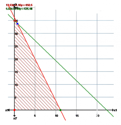
13.531x1+4.16x2≤150.5
5.625x1+3.593x2≤125.48
x1, x2≥0.
The maximum value of the objective function Z=1396.92 occurs at the extreme point (0, 34.92). Hence, the optimal solution to the given LP problem is x1=0, x2=34.92 and max Z=1396.94. and the graphical structure is explained in Figures 2 and 3.
Figure 2. Graphical solution
Figure 3. Graphical structure for feasible and optimal region
Consider a dietary planning scenario involving two types of food items: Food A and Food B. Each gram of Food A provides 20 units of protein and 40 units of minerals, while each gram of Food B supplies 30 units of protein and 30 units of minerals. The nutritional requirements for an individual are assumed to be a minimum of 900 units of protein and 1200 units of minerals per day. The cost per gram of Food A is approximately Rs. 6, and Food B is Rs. 8.
The objective is to determine the optimal quantity (in grams) of each food item to be included in the daily diet such that the total cost is minimized, while satisfying the minimum nutritional requirements. However, it is important to note that both nutritional needs and food prices are subject to variation due to individual health conditions and market fluctuations. To incorporate this uncertainty into the model, the problem is formulated using fuzzy linear programming. Specifically, symmetrical octagonal fuzzy numbers are employed to represent imprecise parameters such as cost and nutritional content.
For instance, the cost of Food A, originally estimated at Rs. 6 per gram, is represented by the symmetrical octagonal fuzzy number (2,3,4,5,7,8,9,10). Similar fuzzy representations are adopted for the remaining uncertain parameters. Based on these fuzzy values, the problem is structured and solved as a fuzzy linear programming model.
$\operatorname{Min} \tilde{Z}=(2,3,4,5,7,8,9,10) \tilde{x}_1+(3,4,5,7,9,11,12,13) \tilde{x}_2$
Subject to
$\begin{gathered}20 \tilde{x}_1+30 \tilde{x}_2 \\ \geq(885,886,888,890,910,912,914,915) 40 \tilde{x}_1+30 \tilde{x}_2 \\ \geq(1190,1191,1193,1195,1205,1207,1209,1210) \\ \tilde{x}_1, \tilde{x}_2 \succ 0\end{gathered}$
Formulating LPP
$\begin{gathered}\operatorname{Min} \tilde{Z}=5.4 \tilde{x}_1+8 \tilde{x}_2 \\ 20 \tilde{x}_1+30 \tilde{x}_2 \geq 900 ; 40 \tilde{x}_1+30 \tilde{x}_2 \geq 1200 \\ \tilde{x}_1, \tilde{x}_2 \succ 0\end{gathered}$
6.1 Doolittle’s method
Using Doolittle’s method in LU decomposition, the constraints can be converted to equation:
$20 x_1+30 x_2=900 ; 40 x_1+30 x_2=1200$
The constraints can be converted into matrix form
$\left[\begin{array}{ll}20 & 30 \\ 40 & 30\end{array}\right]\left[\begin{array}{l}x_1 \\ x_2\end{array}\right]=\left[\begin{array}{c}900 \\ 1200\end{array}\right]$
Now
$\mathrm{A}=\left[\begin{array}{ll}20 & 30 \\ 40 & 30\end{array}\right], \mathrm{X}=\left[\begin{array}{l}x_1 \\ x_2\end{array}\right]$ and $\mathrm{B}=\left[\begin{array}{c}900 \\ 1200\end{array}\right]$
This implies
$\begin{aligned} & u_{11}=20, l_{21} u_{12}+u_{22}=30 ; u_{22}=1.862 \\ & \therefore \mathrm{~A}=\mathrm{LxU}=\mathrm{LU}, \text { let } \mathrm{Ux}=\mathrm{y} \text { then } \mathrm{ly}=\mathrm{B} \\ & y_1, y_2=900,-600\end{aligned}$
Now Ux=y, by using backward method: x2=20, from the above matrix equation
$\begin{aligned} & \mathrm{x}_1=15 \\ & \operatorname{Min} \tilde{Z}=5.4 \tilde{x}_1+8 \tilde{x}_2 \\ & \left(\mathrm{x}_1, \mathrm{x}_2\right)=(15,20) \\ & \operatorname{Min} Z=241\end{aligned}$
Graphical Method
$\begin{gathered}\operatorname{Min} \tilde{Z}=5.4 \tilde{x}_1+8 \tilde{x}_2 ; 20 \tilde{x}_1+30 \tilde{x}_2 \geq 900 \\ 40 \tilde{x}_1+30 \tilde{x}_2 \geq 1200 ; \tilde{x}_1, \tilde{x}_2 \succ 0\end{gathered}$
Figure 4. Graphical solution
Figure 5. Graphical structure for feasible and optimal region for application
$\begin{aligned} & \mathrm{x}_2=20 \\ & \mathrm{x}_1=15 \\ & \operatorname{Min} \tilde{Z}=5.4 \tilde{x}_1+8 \tilde{x}_2 \\ & \left(\mathrm{x}_1, \mathrm{x}_2\right)=(15,20) \\ & \operatorname{Min} Z=241\end{aligned}$
Table 1. Graphical solution
|
Extreme Point Coordinates (x1,x2) |
Lines Through Extreme Point |
Objective Function Value Z=5.4x1+8x2 |
|
A(0,40) |
2→40x1+30x2≥1200 3→x1≥0 |
5.4(0)+8(40)=320 |
|
B(15,20) |
1→20x1+30x2≥900 2→40x1+30x2≥1200 |
5.4(15)+8(20)=241 |
|
C(45,0) |
1→20x1+30x2≥900 4→x2≥0 |
5.4(45)+8(0)=243 |
The maximum value of the objective function Z=241 occurs at the extreme point (15, 20) (Figure 4 and Figure 5). Hence, the optimal solution to the given LP problem is x1 =15, x2 =20 and max Z=241 in Table 1 provided the graphical solution.
A comparative analysis is conducted between the solutions obtained using the existing method and the proposed method. The performance of both methods is evaluated based on their ability to solve the fuzzy linear programming problem and achieve optimal solutions, with a particular focus on the accuracy, efficiency, and reliability of the results in Table 2.
Table 2. The comparative analysis
|
Problems |
Existing Method |
Proposed Method |
|
|
Example 1 |
Max Z=310.882 |
Doolittle’s Method |
Max Z=1396.2 |
|
Simplex Method |
Max Z=1396.94 |
||
|
Graphical Method |
Max Z=1396.94 |
||
|
Application |
Min Z=213 |
Doolittle’s Method |
Min Z=241 |
|
Simplex Method |
Min Z=241 |
||
|
Graphical Method |
Min Z=241 |
||
Versatility Across Domains: The research highlights the broad applicability of Linear Programming (LP) across multiple domains, including agriculture, management, site selection, services, investment, and transportation, which showcases its strategic importance in diverse real-world decision-making contexts.
Incorporation of Octagonal Fuzzy Numbers: The use of Octagonal Fuzzy Numbers (OFNs) allows for more precise modeling of uncertainty, making it easier to handle and represent ambiguous data, thereby enhancing decision-making under uncertainty.
Novel Defuzzification Approach: The introduction of a new defuzzification technique based on a ranking function derived from Pascal’s triangle offers an innovative way to manage the left and right spreads of OFNs, providing a more refined approach for handling fuzzy numbers.
Comparison of Multiple Solution Methods: The study’s comparative analysis of Doolittle’s method, Simplex method, and Graphical method offers a comprehensive evaluation of different approaches, helping to identify the most efficient and optimal solution technique for the given LP problems.
Practical Applicability: The findings emphasize the real-world applicability and efficiency of LP, demonstrating how these methods can be applied to solve complex decision-making problems in various sectors.
Enhanced Decision-Making in Uncertainty: By incorporating octagonal fuzzy numbers, the paper enhances decision-making models, making them more reliable and effective in uncertain environments, which is crucial for real-world applications.
In this research study, the effectiveness of Doolittle's method, the simplex method, and the graphical method in solving linear programming problems under octagonal fuzzy number environments has been systematically examined. A comparative analysis through a numerical example demonstrates that all three methods successfully yield both precise and fuzzy optimal solutions. Notably, Doolittle's method, based on LU decomposition, offers a direct and computationally efficient approach, producing results consistent with those obtained through the simplex and graphical methods. Although a minor error margin is observed with Doolittle’s method, it remains a reliable approximation technique. Owing to its simplicity, computational efficiency, and ease of implementation, Doolittle’s method proves to be a practical and accessible tool for decision-makers handling fuzzy optimization problems.
This study opens several avenues for future research. The application of Doolittle’s method within the framework of fuzzy linear programming can be further extended to accommodate more complex fuzzy environments, such as intuitionistic, Pythagorean, and q-rung orthopair fuzzy sets. Additionally, exploring its integration with advanced multi-objective optimization models under uncertainty can enhance its applicability in real-world decision-making scenarios. Future work may also focus on the development of hybrid algorithms combining Doolittle’s method with metaheuristic or artificial intelligence techniques to improve solution accuracy and computational efficiency. Moreover, the proposed approach can be adapted and validated across diverse domains such as supply chain management, healthcare, finance, and engineering design, where uncertainty and imprecision are inherent.
[1] Tiruneh, A.T., Debessai, T.Y., Bwembya, G.C., Nkambule, S.J. (2019). The LA=U decomposition method for solving systems of linear equations. Journal of Applied Mathematics and Physics, 7(9): 2031. https://doi.org/10.4236/jamp.2019.79140
[2] Pérez-Canedo, B., Verdegay, J.L. (2023). On the application of a lexicographic method to fuzzy linear programming problems. Journal of Computational and Cognitive Engineering, 2(1): 47-56. https://doi.org/10.47852/bonviewJCCE20235142025
[3] Chandrasekaran, S., Gokila, G., Saju, J. (2015). Ranking of octagonal fuzzy numbers for solving multi objective fuzzy linear programming problem with simplex method and graphical method. International Journal of Science, Engineering and Applied Science, 1(5): 504-511. https://ijseas.com/volume1/v1i5/ijseas20150557.pdf
[4] Congedo, M.A. (2022). Tribute to Alan Turing: Symmetric Gaussian elimination. HAL, 4(31). https://hal.science/hal-03660449.
[5] Deshmukh, M., Ghadle, K., Jadhav, O. (2020). An innovative approach for ranking hexagonal fuzzy numbers to solve linear programming problems. International Journal on Emerging Technologies, 11(2): 385-388.
[6] Djordjevic, I., Petrovic, D., Stojic, G. (2019). A fuzzy linear programming model for aggregated production planning (APP) in the automotive industry. Computers in Industry, 110: 48-63. https://doi.org/10.1016/j.compind.2019.05.004
[7] Dong, Y.J., Wan, S.P. (2018). A new trapezoidal fuzzy linear programming method considering the acceptance degree of fuzzy constraints violated. Knowledge-Based Systems, 148: 100-114. https://doi.org/10.1016/j.knosys.2018.02.030
[8] Gani, A.N., Duraisamy, C., Veeramani, C. (2009). A note on fuzzy linear programming problem using LR fuzzy number. International Journal of Algorithms, Computing and Mathematics, 2(3): 93-106.
[9] Ghadle, K.P., Ingle, S.M. (2018). A new ranking on generalized octagonal fuzzy numbers. International Journal of Applied Engineering Research, 13(16): 12702-12709. https://doi.org/10.35940/ijeat.c5741.029320
[10] Gurukumaresan, D., Duraisamy, C., Srinivasan, R. (2021). Optimal solution of fuzzy transportation problem using octagonal fuzzy numbers. Computer Systems Science & Engineering, 37(3). https://doi.org/10.32604/csse.2021.014130
[11] Garg, H. (2018). A linear programming method based on an improved score function for interval-Valued Pythagorean fuzzy numbers and its application to decision-Making. International Journal of Uncertainty, Fuzziness and Knowledge-Based Systems, 26(1): 67-80. https://doi.org/10.1142/S0218488518500046
[12] Kumar, R., Dhiman, G. (2021). A comparative study of fuzzy optimization through fuzzy number. International Journal of Modern Research, 1(1): 1-14. http://doi.org/10.37896/jxu14.6/173
[13] Kurian, B. (2024). Cognitive rehabilitation-game therapy. In 2024 International Conference on Advances in Computing, Communication and Applied Informatics (ACCAI), Chennai, India, pp. 1-5. https://doi.org/10.1109/ACCAI61061.2024.10601764
[14] Maiti, I., Mandal, T., Pramanik, S., Das, S.K. (2021). Solving multi-objective linear fractional programming problem based on Stanojevic's normalisation technique under fuzzy environment. International Journal of Operational Research, 42(4): 543-564. https://doi.org/10.1504/IJOR.2021.119941
[15] Malini, S.U., Kennedy, F.C. (2013). An approach for solving fuzzy transportation problem using octagonal fuzzy numbers. Applied Mathematical Sciences, 7(54): 2661-2673.
[16] Meenakshi, K., Sathish, S. (2024). Non overlapping fuzzy octagonal numbers for recommending the optimum equity value of financial series. Global & Stochastic Analysis, 11(3).
[17] Meili, Y., Yaping, D., Qingsheng, W., Yibo, G., Xin, L., Xiangjing, B. (2009). Analysis of blend spectra of nitrophenol isomers with Doolittle multivariate calibration. Journal of the Iranian Chemical Research. Unspecified Source, 23-29.
[18] Muralidaran, C., Venkateswarlu, B. (2017). Accuracy ranking function for solving hexagonal fuzzy linear programming problem. International Journal of Pure and Applied Mathematics, 115: 215-222.
[19] Mittal, R.C., Kurdi, A.A. (2002). Efficient solution of a sparse non-symmetric system of linear equations. International Journal of Computer Mathematics, 79(4): 449-463. https://doi.org/10.1080/00207160210940
[20] Pandian, P., Jayalakshmi, M. (2010). A new method for solving integer linear programming problems with fuzzy variables. Applied Mathematical Sciences, 4(20): 997-1004.
[21] Praveen Prakash, A., Geetha Lakshmi, M. (2018). Sub-Trident form using fuzzy aggregation. International Journal of Engineering Sciences & Research Technology, 5.
[22] Rafique, M. (2015). The solution of a system of linear equations by an improved LU-Decomposition method. American Journal of Scientific and Industrial Research, Science Huβ. https://doi.org/10.5251/ajsir.2015.6.2.23.24
[23] Darvishi Salookolaei, D., Nasseri, S.H. (2020). A dual simplex method for grey linear programming problems based on duality results. Grey Systems: Theory and Application, 10(2): 145-157. https://doi.org/10.1108/GS-10-2019-0044
[24] Sanei, M. (2013). The simplex method for solving fuzzy number linear programming problem with bounded variable. Journal of Basic and Applied Scientific Research, 3(3): 618-625.
[25] Saxena, P., Jain, R. (2019). Bector-Chandra type duality in linear programming under fuzzy environment using hyperbolic tangent membership functions. International Journal of Fuzzy System Applications, 8(2): 68-88. https://doi.org/10.4018/IJFSA.2019040104
[26] Someshwar, S. (2020). Solving fuzzy LPP for pentagonal fuzzy number using ranking approach. Mukt Shabd Journal, 9.
[27] Dinagar, D.S., Jeyavuthin, M.M. (2018). A note on integer linear programming problems with LR pentagonal fuzzy numbers. Journal of Computer and Mathematical Sciences, 9(9): 1093-1100. https://doi.org/10.29055/JCMS%2F848
[28] Stephen, D.D., Jeyavuthin, M.M. (2019). Distinct methods for solving fully fuzzy linear programming problems with pentagonal fuzzy number. Journal of Computer and Mathematical Sciences, 10(6): 1253-1260.
[29] Suba, M., Osman, W.M., Ibrahim, T.F. (2024). Octagonal fuzzy DEMATEL approach to study the risk factors of stomach cancer. Journal of Computational Analysis & Applications, 32(1).
[30] Sudha, A., Sahaya, M., Revathy, M. (2016). A new ranking on hexagonal fuzzy numbers. International Journal of Fuzzy Logic Systems, 6(4): 1-8. https://doi.org/10.5121/ijfls.2016.6401
[31] Vivekanand, V., Prakash, G.S. (2019). Application of deterministic, stochastic and fuzzy linear programming models in solid waste management studies: Literature review. The Journal of Solid Waste Technology and Management, 45(1): 68-75. https://doi.org/10.5276/JSWTM.2019.68
[32] Zandkarimkhani, S., Mina, H., Biuki, M., Govindan, K. (2020). A chance constrained fuzzy goal programming approach for perishable pharmaceutical supply chain network design. Annals of Operations Research, 295: 425-452. https://doi.org/10.1007/s10479-020-03677-7
[33] Zimmermann, H.J. (1993). Applications of fuzzy set theory to mathematical programming. Readings in Fuzzy Sets for Intelligent Systems, 795-809. https://doi.org/10.1016/B978-1-4832-1450-4.50084-5