Youb Okkacha*![]() | Djoudi Warda
| Djoudi Warda![]() | Bouarfa Said
| Bouarfa Said![]()
© 2025 The authors. This article is published by IIETA and is licensed under the CC BY 4.0 license (http://creativecommons.org/licenses/by/4.0/).
OPEN ACCESS
The Functional Variable Algorithm (FVA) is a new approach to solving nonlinear partial differential equations. Benjamin-Bona-Mahony (BBM) equation addresses a fundamental model for long-wave propagation in nonlinear dispersive systems. Explicit traveling wave solutions comprising solitary waves and periodic groups can be derived using methodical mathematical techniques and symbolic computation. Unlike other techniques, such as the inverse scattering transform or tanh–coth methods, the FVA depends on transforming the functional variable, i.e., simplifying the functions' derivatives. It made it easier for us to find the solution, as we obtained eight solutions for each equation in two uniform forms, periodic and solitary wave solutions, unlike tanh–coth methods, which obtained a small number of non-uniform solutions: periodic and solitary and compaction solutions; This means this method has greater computational efficiency and freedom than other methods. Designed to unite the answers obtained, the General Mathematical Model of Waveforms (GMMW) offer a framework for analyzing nonlinear wave events. The results show that the FVA technique is quite efficient and generally applicable in different fields, including optical communications, nonlinear physics, and fluid dynamics.
nonlinear equations, Functional Variable Algorithm, traveling wave solutions, Benjamin-Bona-Mahony equation, analytical methods
Nonlinear partial differential equations (NPDEs) commonly model complex behavior in optical communications and fluid mechanics fields [1-3]. It is essential to look at traveling wave solutions when studying things like dispersion, the behavior of soliton particles, and periodic events in nonlinear media [4]. Despite the significant advancements in numerical simulations, obtaining a robust analytical solution remains challenging due to the numerous nonlinearities and the dependence of iterative numerical methods on the initial conditions [5]. In the past decades, many analytical techniques have been devised to solve NPDEs. Traditional methods like the inverse scattering transform, tanh–coth methods, extended tanh-function methods, sine–cosine methods, and homogeneous balance techniques have helped us learn much about these systems [6-8]. However, many of these approaches either suffer from limitations regarding their range or in their representation of the complete solution space, especially when it comes to complicated, nonlinear equations [9]. In this context, we present the Functional Variable Algorithm (FVA), a new methodology we have developed and optimized. Using a new set of theoretical insights, the FVA provides a systematic mathematical series of transformations that put NPDEs into forms that are easier to work [10-12]. The FVA allows symbolic computation tools like Mathematica to build explicit forms for solitary and periodic traveling wave solutions [13-15]. We use the standard FVA to solve the Benjamin-Bona-Mahony (BBM) equation for long-wave propagation in media that scatters them [16]. We provide new theoretical results that give the basis for the method and offer a full-fledged mathematical model General Mathematical Model of Waveforms (GMMW) for both solutions found [17, 18]. Besides broadening the NPDE analytical toolbox, this work paves the way for future investigations of intricate nonlinear processes across various scientific fields [19, 20].
2.1 An exposition of the FVA
An exposition of the FVA:
This section provides a detailed presentation of the FVA used to obtain analytical solutions for nonlinear equations. Our approach is organized into several identified steps, ranging from the transformation of the original equation to its final integration. This formulation ensures reproducibility by other researchers. It is important to recall that the primary objective is to derive precise solutions for equations such as BBM equation.
Step 1: We introduce the ordinary differential equation (ODE), which can be stated as multiple independent variables.
$\Upsilon\left(U, U_{\xi}, U_{\xi \xi}, U_{\xi \xi \xi}, U_{\xi \xi \xi \xi}, \ldots.\right)$ (1)
$\Upsilon$ represents a set of functions, $U(\xi)$ denotes a traveling wave function that needs to be ascertained, and $\xi$ represents a wave variable:
$\xi_n=n d+C t+\delta$ (2)
In this context, $n$ represents the discrete variable, while $C$ denotes the velocity. The constants $d$ and $\delta$ are arbitrary.
$u(x, t)=U(\xi)$ (3)
$U^{\prime}(\xi)=U \xi=f(\xi)$ (4)
Step 2: Transformation via the functional variable
Next, we express f(ξ) in terms of a functional variable using an appropriate transformation:
$\mathrm{f}(\xi)=\mathrm{h}(\varphi(\xi))$ (5)
where, φ(ξ) is the new functional variable, h is a function that simplifies the equation.
Step 3: Calculation of derivatives and substitutions
The successive derivatives of f(ξ) concerning ξ are computed using the chain rule. For instance, the first derivative is given by:
$U^{\prime \prime}(\xi)=U \xi \xi=f^{\prime}(\xi)=h^{\prime}(\varphi(\xi)) \cdot \varphi^{\prime}(\xi)$ (6)
And similarly for higher-order derivatives. These expressions are then substituted back into the ODE (1), reducing the equation to a form involving only φ(ξ) and its derivatives.
Step 4: Reduction and integration process
After substitution and algebraic manipulation, the equation is simplified to a new expression:
$\varepsilon\left(\varphi, \varphi^{\prime}, \varphi^{\prime \prime}\right)=0$ (7)
In many cases, Eq. (7) is integrable using standard methods (e.g., separation of variables or by finding an integrating factor). By integrating Eq. (7) with a clear justification for any constant(s) of integration (often set to zero as an initial simplifying assumption), the desired analytical solution for f(ξ) is ultimately obtained.
2.2 Reproducibility of the methodology
To ensure that other researchers can replicate our results, we provide the following pseudo-code outlining the steps of the FVA:
1. Define the initial ODE:
Input the general Eq. (1) and apply the transformation u(x, t) = u(ξ) with ξ = x − ct.
2. Perform the variable transformation:
Set f(ξ) = h(φ(ξ)) and calculate the derivatives using the chain rule.
3. Substitute and simplify:
Replace f(ξ) and its derivatives in (1) to obtain the transformed Eq. (7).
4. Integrate:
Integrate Eq. (7) while justifying the choice of integration constants (setting them to zero initially).
5. Verify and validate:
Compare the obtained solution with a known test case or analytical solution to ensure the method’s correctness.
2.3 Illustrative example on a simple case
Before applying the FVA to the complete BBM model, we provide a brief illustration using a simplified nonlinear ODE, such as:
$U^{\prime \prime}(\xi)+k \cdot[U(\xi)]^2=0$ (8)
For this example, the same steps described above are followed:
1. Adopt the transformation $U \xi=f(\xi)=h(\varphi(\xi))$.
2. Compute the derivatives and substitute into the ODE.
3. Integrate and simplify.
$f^{\prime}(\xi)+k \cdot\left[\int f(\xi)\right]^2=0$ (9)
$h^{\prime}(\varphi(\xi)) \cdot \varphi^{\prime}(\xi)+k \cdot\left[\int h(\varphi(\xi))\right]^2=0$ (10)
This example demonstrates the FVA's clarity and robustness before it is applied to more complex systems.
The findings above were previously acquired using the BBM equation. The equation presented here is a mathematical model that describes the behavior of long waves in nonlinear dispersive systems.
So, the form of the BBM for every order is Eq. (11) and Eq. (37)
Example 1:
According to BBM equation,
$\left(U^n\right)_t-\left(U^n\right)_{X X X}+B\left(U^m\right)_X=0, n>m>1$ (11)
Case 1: If $\xi=X-C t+\xi_0$ and $V=U^m$, we achieve
$-C\left(V^{\frac{n}{m}}\right)_{\xi}-\left(V^{\frac{n}{m}}\right)_{\xi \xi \xi}+\beta(V)_{\xi}=0$ (12)
$\beta$ and $C$ are the constant and the velocity, after integrating Eq. (12) once concerning ξ, set the integration constants to zero and combining both equations yields the simplified form
$-\frac{c m}{n+m}\left(v^{\frac{n}{m}+1}\right)-\frac{1}{2}\left(\left(v^{\frac{n}{m}}\right)_{\xi}\right)^2+\frac{\alpha}{2}\left(v^2\right)=0$ (13)
According to Eq. (3) and Eq. (4), and after simplifying Eq. (13), the expression becomes:
$\mathrm{f}(\xi)=\left(V^{\frac{n}{m}}\right)_{\xi}=V \sqrt{\alpha} \sqrt{1-\frac{2 c V^{-1+\frac{n}{m}}}{\alpha\left(1+\frac{n}{m}\right)}}$ (14)
Depending on the Eq. (12), the differential Eq. (7) was completely integrable since its solutions were deduced from the integral:
$\int \frac{d s}{s \sqrt{1-s}}=\ln \left|\frac{1-\sqrt{1-s}}{1+\sqrt{1-s}}\right|$ (15)
So that
$\int f(\xi)=\int \frac{\left(V^{\frac{n}{m}}\right)_{\xi}}{V \sqrt{\alpha} \sqrt{1-\frac{2 c V^{-1+\frac{n}{m}}}{\alpha\left(1+\frac{n}{m}\right)}}}$ (16)
By looking at Eq. (4) and the relation Eq. (16), the following quadratic equation is obtained as follows:
$W^2 Z^2+4\left(1-W^2\right) Z-4\left(1-W^2\right)=0$ (17)
where,
$W=\frac{2 \tan ^2\left[\frac{1}{2}\left(-1+\frac{n}{m}\right) \sqrt{\beta} \xi\right]}{1+\tan ^2\left[\frac{1}{2}\left(-1+\frac{n}{m}\right) \sqrt{\beta} \xi\right]}$ (18)
And
$Z=\frac{2 C V^{-1+\frac{n}{m}}}{\left(1+\frac{n}{m}\right) \beta}$ (19)
After performing a basic algebraic manipulation, the two solutions of Eq. (12) can be obtained.
For $\beta>0$:
$V_1[\xi]=2^{-\frac{1}{-1+\frac{n}{m}}}\left(\frac{\left.\left(1+\frac{n}{m}\right) \beta \operatorname{sech} \frac{1}{2}\left(-1+\frac{n}{m}\right) \sqrt{\beta} \xi\right]}{C}\right)^{\frac{1}{-1+\frac{n}{m}}}$ (20)
$V_2[\xi]=2^{-\frac{1}{-1+\frac{n}{m}}}\left(-\frac{\left.\left(1+\frac{n}{m}\right) \beta \operatorname{csch} \frac{1}{2}\left(-1+\frac{n}{m}\right) \sqrt{\beta} \xi\right]}{C}\right)^{\frac{1}{-1+\frac{n}{m}}}$ (21)
For $\beta<0$:
$V_1[\xi]=2^{-\frac{1}{-1+\frac{n}{m}}}\left(\frac{\left.\left(1+\frac{n}{m}\right) \beta \sec \frac{1}{2}\left(-1+\frac{n}{m}\right) \sqrt{-\beta} \xi\right]}{C}\right)^{\frac{1}{-1+\frac{n}{m}}}$ (22)
$V_2[\xi]=2^{-\frac{1}{-1+\frac{n}{m}}}\left(-\frac{\left.\left(1+\frac{n}{m}\right) \beta \csc \frac{1}{2}\left(-1+\frac{n}{m}\right) \sqrt{-\beta} \xi\right]}{C}\right)^{\frac{1}{-1+\frac{n}{m}}}$ (23)
We have $U[x]=V^{\frac{1}{m}}[x]$, so:
For $\beta>0$: We obtain the following solitary wave solutions
$U_1[\xi]=2^{-\frac{1}{\mathrm{n}-\mathrm{m}}}\left(\frac{\left.\left(1+\frac{n}{m}\right) \beta \operatorname{sech} \frac{1}{2}\left(-1+\frac{n}{m}\right) \sqrt{\beta} \xi\right]}{C}\right)^{\frac{1}{\mathrm{n}-\mathrm{m}}}$ (24)
$U_2[\xi]=2^{-\frac{1}{n-m}}\left(-\frac{\left.\left(1+\frac{n}{m}\right) \beta \operatorname{csch} \frac{1}{2}\left(-1+\frac{n}{m}\right) \sqrt{\beta} \xi\right]}{C}\right)^{\frac{1}{n-m}}$ (25)
For $\beta<0$: We obtain the following the periodic wave solutions
$U_1[\xi]=2^{-\frac{1}{n-m}}\left(\frac{\left.\left(1+\frac{n}{m}\right) \beta \sec \frac{1}{2}\left(-1+\frac{n}{m}\right) \sqrt{-\beta} \xi\right]}{C}\right)^{\frac{1}{n-m}}$ (26)
$U_2[\xi]=2^{-\frac{1}{n-m}}\left(-\frac{\left.\left(1+\frac{n}{m}\right) \beta \csc \frac{1}{2}\left(-1+\frac{n}{m}\right) \sqrt{-\beta} \xi\right]}{C}\right)^{\frac{1}{n-m}}$ (27)
Case 2: If $\xi=X-C t+\xi_0$ and $V=U^n$ Eq. (11) becomes the ODE:
$-C(V)_{\xi}-(V)_{\xi \xi \xi}+\alpha(V)_{\xi}=0$ (28)
Two solutions are obtained through straightforward algebraic manipulation:
For $C$>0
$V_1[\xi]=2^{-\frac{n}{m-n}}\left(\frac{\left.C\left(1+\frac{m}{n}\right) \operatorname{sech} \frac{1}{2} \sqrt{C}\left(-1+\frac{m}{n}\right) \xi\right]}{\beta}\right)^{\frac{n}{m-n}}$ (29)
$V_2[\xi]=2^{-\frac{n}{m-n}}\left(-\frac{\left.C\left(1+\frac{m}{n}\right) \operatorname{csch} \frac{1}{2} \sqrt{C}\left(-1+\frac{m}{n}\right) \xi\right]}{\beta}\right)^{\frac{n}{m-n}}$ (30)
For $C$<0:
$V_1[\xi]=2^{-\frac{n}{m-n}}\left(\frac{\left.C\left(1+\frac{m}{n}\right) \sec \frac{1}{2} \sqrt{-C}\left(-1+\frac{m}{n}\right) \xi\right]}{\beta}\right)^{\frac{n}{m-n}}$ (31)
$V_2[\xi]=2^{-\frac{n}{m-n}}\left(-\frac{\left.C\left(1+\frac{m}{n}\right) \csc \frac{1}{2} \sqrt{-C}\left(-1+\frac{m}{n}\right) \xi\right]}{\beta}\right)^{\frac{n}{m-n}}$ (32)
We have $U[\xi]=V[\xi]^{\frac{1}{n}}$, so:
For $C$>0:
$U_1[\xi]=2^{-\frac{1}{m-n}}\left(\frac{\left.C\left(1+\frac{m}{n}\right) \operatorname{sech} \frac{1}{2} \sqrt{C}\left(-1+\frac{m}{n}\right) \xi\right]}{\beta}\right)^{\frac{1}{m-n}}$ (33)
$U_2[\xi]=2^{-\frac{1}{m-n}}\left(-\frac{\left.C\left(1+\frac{m}{n}\right) \operatorname{csch} \frac{1}{2} \sqrt{C}\left(-1+\frac{m}{n}\right) \xi\right]}{\beta}\right)^{\frac{1}{m-n}}$ (34)
For $C$<0:
$U_1[\xi]=2^{-\frac{1}{m-n}}\left(\frac{\left.C\left(1+\frac{m}{n}\right) \sec \frac{1}{2} \sqrt{-C}\left(-1+\frac{m}{n}\right) \xi\right]}{\beta}\right)^{\frac{1}{m-n}}$ (35)
$U_2[\xi]=2^{-\frac{1}{m-n}}\left(-\frac{\left.C\left(1+\frac{m}{n}\right) \csc \frac{1}{2} \sqrt{-C}\left(-1+\frac{m}{n}\right) \xi\right]}{\beta}\right)^{\frac{1}{m-n}}$ (36)
Example 2:
the complexity of BBM equations to analyze and numerically work on motivation; we employ our technique on the complexity of BBM equation. It involves balancing the expression convection $U^m U_X$ and the expression dispersion $(U^n )_XXX$, as described in reference.
According to the generalized BBM equation
$\begin{gathered}\left(U^n\right)_t+\left(U^n\right)_X-\left(U^n\right)_{X X X}+a(m+1) U^m(U)_X=0,\ n>m>1\end{gathered}$ (37)
Case 1: If $\xi=X-C t+\xi_0$ and $V=U^{m+1}$, we obtain
$(-C+1)\left(V^{\frac{n}{m+1}}\right)_{\xi}-\left(V^{\frac{n}{m+1}}\right)_{\xi \xi \xi}+\beta(V)_{\xi}=0$ (38)
Following the same procedure and some straightforward algebraic manipulations, the following solutions are obtained:
For β>0:
$V_1[\xi]=\left(\frac{\left.-\beta\left(\frac{n}{m+1}+1\right) \operatorname{sech} \frac{1}{2} \sqrt{\beta}\left(-1+\frac{n}{m+1}\right) \xi\right]}{2(1-C)}\right)^{\frac{1}{\left(\frac{n}{m+1}-1\right)}}$ (39)
$V_2[\xi]=\left(\frac{\left.\beta\left(\frac{n}{m+1}+1\right) \operatorname{csch} \frac{1}{2} \sqrt{\beta}\left(-1+\frac{n}{m+1}\right) \xi\right]}{2(1-C)}\right)^{\frac{1}{\left(\frac{n}{m+1}-1\right)}}$ (40)
$V_1[\xi]=\left(\frac{\left.-\beta\left(\frac{n}{m+1}+1\right) \sec \frac{1}{2} \sqrt{-\beta}\left(-1+\frac{n}{m+1}\right) \xi\right]}{2(1-C)}\right)^{\frac{1}{\left(\frac{n}{m+1}-1\right)}}$ (41)
$V_2[\xi]=\left(\frac{\left.\beta\left(\frac{n}{m+1}+1\right) \csc \frac{1}{2} \sqrt{-\beta}\left(-1+\frac{n}{m+1}\right) \xi\right]}{2(1-C)}\right)^{\frac{1}{\left(\frac{n}{m+1}-1\right)}}$ (42)
We have $U[\xi]=V^{\frac{1}{m+1}}[\xi]$, so:
For $\beta>0$, we obtain the following solitary solutions:
$U_1[\xi]=\left(-\frac{\left.\beta\left(\frac{n}{m+1}+1\right) \operatorname{sech} \frac{1}{2} \sqrt{\beta}\left(-1+\frac{n}{m+1}\right) \xi\right]}{2(1-C)}\right)^{\frac{1}{(n-m-1)}}$ (43)
$U_2[\xi]=\left(\frac{\left.\beta\left(\frac{n}{m+1}+1\right) \operatorname{csch} \frac{1}{2} \sqrt{\beta}\left(-1+\frac{n}{m+1}\right) \xi\right]}{2(1-C)}\right)^{\frac{1}{(n-m-1)}}$ (44)
For $\beta<0$:
$U_1[\xi]=\left(-\frac{\left.\beta\left(\frac{n}{m+1}+1\right) \sec \frac{1}{2} \sqrt{-\beta}\left(-1+\frac{n}{m+1}\right) \xi\right]}{2(1-C)}\right)^{\frac{1}{(n-m-1)}}$ (45)
$U_2[\xi]=\left(\frac{\left.\beta\left(\frac{n}{m+1}+1\right) \csc \frac{1}{2} \sqrt{-\beta}\left(-1+\frac{n}{m+1}\right) \xi\right]}{2(1-C)}\right)^{\frac{1}{(n-m-1)}}$ (46)
Case 2: If $\xi=X-C t+\xi_0$ and $V=U^n$, Eq. (37) becomes the ODE:
$(-C+1)(V)_{\xi}-(V)_{\xi \xi \xi}+\beta\left(V^{\frac{m+1}{n}}\right)_{\xi}=0$ (47)
We obtain two solutions after some simple algebraic manipulation:
For $1-C>0$:
$V_1[\xi]=\left(-\frac{\left.(1-C)\left(\frac{m+1}{n}+1\right) \operatorname{sech} \frac{(\sqrt{(1-C)}}{2}\left(\frac{m+1}{n}-1\right) \xi\right]}{2 \beta}\right)^{\frac{n}{(m+1-n)}}$ (48)
$V_2[\xi]=\left(\frac{\left.(1-C)\left(\frac{m+1}{n}+1\right) \operatorname{csch} \frac{(\sqrt{(1-C)}}{2}\left(\frac{m+1}{n}-1\right) \xi\right]}{2 \beta}\right)^{\frac{n}{(m+1-n)}}$ (49)
For $1-C<0$:
$V_1[\xi]=\left(\frac{\left.(1-C)\left(\frac{m+1}{n}+1\right) \sec \frac{(\sqrt{-(1-C)}}{2}\left(\frac{m+1}{n}-1\right) \xi\right]}{2 \beta}\right)^{\frac{n}{(m+1-n)}}$ (50)
$V_2[\xi]=\left(\frac{\left.(1-C)\left(\frac{m+1}{n}+1\right) \csc \frac{(\sqrt{-(1-C)}}{2}\left(\frac{m+1}{n}-1\right) \xi\right]}{2 \beta}\right)^{\frac{n}{(m+1-n)}}$ (51)
We have $U[\xi]=V^{\frac{1}{n}}[\xi]$, so:
For $1-C>0$:
$U_1[\xi]=2^{\frac{-1}{1+m-n}}\left(\frac{(1-C)\left(\frac{m+1}{n}+1\right) \operatorname{sech} \frac{(\sqrt{(1-C)}}{2}\left(\frac{m+1}{n}-1\right) \xi}{\beta}\right)^{\frac{1}{(m+1-n)}}$ (52)
$U_2[\xi]=2^{\frac{-1}{1+m-n}}\left(\frac{\left.(1-C)\left(\frac{m+1}{n}+1\right) \operatorname{csch} \frac{(\sqrt{(1-C)}}{2}\left(\frac{m+1}{n}-1\right) \xi\right]}{\beta}\right)^{\frac{1}{(m+1-n)}}$ (53)
For $1-C<0$:
$U_1[\xi]=2^{\frac{-1}{1+m-n}}\left(-\frac{\left.(1-C)\left(\frac{m+1}{n}+1\right) \sec \frac{(\sqrt{-(1-C)}}{2}\left(\frac{m+1}{n}-1\right) \xi\right]}{\beta}\right)^{\frac{1}{(m+1-n)}}$ (54)
$U_2[\xi]=2 \frac{-1}{1+m-n}\left((1-C)\left(\frac{m+1}{n}+1\right) \frac{\csc ^2\left[\frac{(\sqrt{-(1-C)}}{2}\left(\frac{m+1}{n}-1\right) \xi\right]}{\beta}\right)^{\frac{1}{(m+1-n)}}$ (55)
Two principal notes emerge from these transformation schemes:
Note 1: delineates the conditions required to obtain solitary wave solutions. The subsequent algebraic manipulations and integration steps lead to quadratic equations whose solutions (as represented in Eqs. (24), (25), (33), (34), (43), (44), (52), (53) correspond to distinct branches of solitary wave profiles.
Note 2: addresses the derivation of periodic wave solutions. Through similar algebraic procedures and integration (illustrated by Eqs. (26), (27), (35), (36), (45), (46), (54), (55), periodic solutions are derived, offering an alternative analytical description of the nonlinear dynamics.
These derivations confirm that the FVA simplifies the solution process and clearly distinguishes between solitary and periodic wave systems.
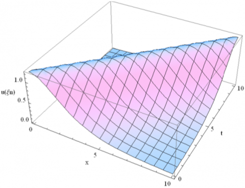
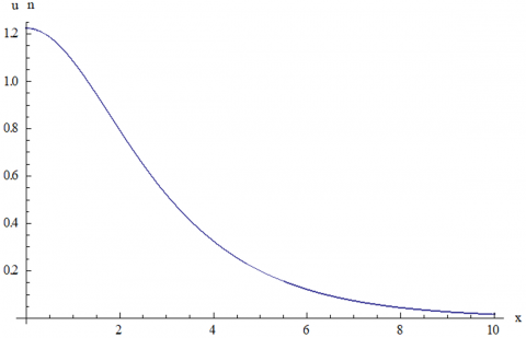
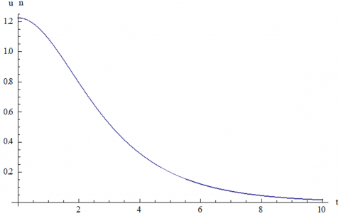
Symbolic computation was performed using Mathematica to validate the analytical results. For example, Figures 1-3 illustrate the solitary wave profile obtained from the derived Eq. (24). In this graphical representation, specific parameter values $(\beta>0, n=4, m=2, \beta=1, C=1)$ were chosen to depict the solitary structure accurately. The smooth transition in numerical plots further substantiates the integration process's robustness and confirms the derived solutions' internal consistency.
Figure 1. Plot 3D representation of Eq. (24)
Figure 2. Plot 2D representation of Eq. (24) for t =0
Figure 3. Plot 2D representation of Eq. (24) for x=0
After substituting the specific parameter values into Eq. (24), the simplified form is as follows:
$U_1[\xi]=U_1[x-t]=2^{-\frac{1}{2}}\left(\frac{3 \operatorname{sech}^2\left[\frac{1}{2}(x-t)\right]}{1}\right)^{\frac{1}{2}}$ (56)
The GMMW, an innovative class of explicit exact solutions to BBM equations, is obtained through the FVA via a non-singular combination of the functioning described by:
$U[\xi]=\left(\frac{A F^2[B \xi]}{M}\right)^N$ (57)
In which $F$ denotes a widely recognized and suitable function.
A is a specific parameter in this article that is related to: C, n,m, $\beta$.
M is a specific parameter in this article that is related to: C, $\beta$.
B is a specific parameter in this article that is related to: C, n,m, $\beta$.
N is specifically the exponent in this article that is related to: n,m.
Compared to conventional analytical techniques—such as the inverse scattering transform, the tanh–coth method [21-23], and the homogeneous balance method.
We notice they studied the same types of nonlinear equations of BBM, which gave non-uniform solutions, compaction, and solitary solutions, using the unified algebraic method with symbolic computation in each BBM equation (11) and (37). However, we find eight types of exact traveling wave solutions in two uniform forms: four periodic solutions and four solitary wave solutions that prove the effectiveness and strength of the function variable method.
The FVA offers distinct advantages. Notably:
- The FVA provides a unified framework for obtaining solitary and periodic wave solutions in closed form, whereas traditional methods often focus exclusively on one type.
- Our method saves time in finding solutions, unlike other analytical methods.
- Unlike iterative numerical techniques, which are highly sensitive to initial conditions, the FVA presents analytical solutions derived directly from the governing equations.
- The method’s ability to generate a general mathematical model (GMMW) enhances its potential for application across a wide range of nonlinear systems.
These comparative advantages highlight the FVA as a robust alternative for researchers seeking precise analytical characterizations of nonlinear wave phenomena.
This work presents and extensively validates a new FVA to find explicit traveling wave solutions for the BBM equation. Four separate analytical solutions, including solitary and periodic waves, have been derived using a methodical procedure of mathematical transformations, derivative computations via the chain rule, and strategic integration.
A significant contribution of this study is the formulation of a GMMW, which captures the whole set of solutions obtained with the FVA. This unified framework is more practical than previous methods, such as the inverse scattering transform and the tanh–coth approach since it simplifies the analysis of nonlinear dispersive systems. Specifically, the FVA's methodical approach and simplicity of use produce exact and repeatable closed-form answers.
Moreover, the method's generality suggests that it could be extended to other complex nonlinear evolution equations encountered in fluid dynamics, optical communications, and climate modeling.
While the current study demonstrates the efficacy of the FVA in deriving exact traveling wave solutions for the BBM equation, several avenues remain for future exploration:
• A detailed parametric study could optimize the choice of functional transformations, enhancing the solutions' physical fidelity.
• Integrating of the FVA with numerical simulations may provide a hybrid framework, combining the precision of analytical methods with the flexibility of computational approaches.
• Extending the methodology to address higher-dimensional or more complex nonlinear systems could broaden its application scope.
In summary, the FVA successfully produces analytical solutions and offers a clear pathway for future advancements in the mathematical modeling of nonlinear phenomena.
We want to thank CRSTRA (Scientific and Technical Research Center on Arid Regions, Biskra), at Mohamed Khider University for its support.
|
f(ξ) |
Terms of a functional variable |
|
φ(ξ) |
The new functional variable |
|
h |
Function is chosen to simplify the equation |
|
A |
The set of functions considered in the analytical model. |
|
BBM |
Abbreviation for the Benjamin–Bona–Mahony equation, a mathematical model that delineates the propagation of long waves in nonlinear dispersive systems. |
|
c |
The wave propagation speed is determined by the characteristics of the medium and the phenomenon under investigation. |
|
FVA |
Functional Variable Algorithm is a method employed to transform certain nonlinear partial differential equations into analytically manageable ordinary differential equations. |
|
f |
A generic function that represents specific behaviors within the model. |
|
GMMW |
General Mathematical Model of Waveforms, a unified framework encompassing all analytical solutions obtained using the FVA. |
|
NPDE(s) |
Nonlinear partial differential equations that model complex phenomena across various fields. |
|
n |
A discrete variable (or index) appears in the model expression or the numerical discretization process. |
|
u |
The traveling wave function to be determined, e.g., representing the profile of a disturbance in the system. |
|
Greek symbols |
|
|
$\alpha$ |
An arbitrary constant is introduced during transformations or integrations. |
|
$\beta$ |
An arbitrary constant is introduced during transformations or integrations. |
|
ξ |
The wave variable (often defined as ξ = x – c·t) transforms the equation into an autonomous form by grouping spatial and temporal dependencies. |
[1] Wang, K.J. (2020). A variational principle for the (3+1)-dimensional extended quantum Zakharov-Kuznetsov equation in plasma physics. Europhysics Letters, 132(4): 44002. https://doi.org/10.1209/0295-5075/132/44002
[2] Wang, K.J., Li, S. (2024). Complexiton, complex multiple kink soliton and the rational wave solutions to the generalized (3+1)-dimensional Kadomtsev-Petviashvili equation. Physica Scripta, 99(7): 075214. https://doi.org/10.1088/1402-4896/ad5062
[3] Vitanov, N.K. (2019). New developments of the methodology of the modified method of simplest equation with application. arXiv preprint arXiv:1904.03481. https://doi.org/10.48550/arXiv.1904.03481
[4] Rueda-Bayona, J.G., Carrillo, J., Cabello Eras, J.J. (2023). The wind-current-water levels effect over surface wave parameters nearby the Magdalena River delta: A numerical approach. Mathematical Modelling of Engineering Problems, 10(3): 993-1002. https://doi.org/10.18280/mmep.100333
[5] Zeki, M., Tatar, S. (2023). An iterative approach for numerical solution to the time-fractional Richards equation with implicit Neumann boundary conditions. European Journal of Pure and Applied Mathematics, 16(1): 491-502. https://doi.org/10.29020/nybg.ejpam.v16i1.4679
[6] Abdoon, M.A., Hasan, F.L. (2022). Advantages of the differential equations for solving problems in mathematical physics with symbolic computation. Mathematical Modelling of Engineering Problems, 9(1): 268-276. https://doi.org/10.18280/mmep.090133
[7] Serrat, A., Djebbar, B. (2022). Solving symmetrical drop suspended equilibrium equation by artificial bee colony programming. Mathematical Modelling of Engineering Problems, 9(2): 507-514. https://doi.org/10.18280/mmep.090229
[8] Ibrahim, I.A., Taha, W.M., Alobaidi, M., Jameel, A.F., Bashier, E., Alshirawi, N.H. (2024). Oblique closed form solution for some type fractional evolution equations in physical problem by using the homogeneous balance method. Mathematical Modelling of Engineering Problems, 11(1): 185-191. https://doi.org/10.18280/mmep.110120
[9] Hanif, Y., Saleem, U. (2023). On multi-hump solutions of reverse space-time nonlocal nonlinear Schrödinger equation. Physica Scripta, 98(6): 065211. https://doi.org/10.1088/1402-4896/acd1c4
[10] Kenefake, D., Armingol, E., Lewis, N.E., Pistikopoulos, E.N. (2022). An improved algorithm for flux variability analysis. BMC Bioinformatics, 23(1): 550. https://doi.org/10.1186/s12859-022-05089-9
[11] van der Zwaard, T., Grzelak, L.A., Oosterlee, C.W. (2022). Relevance of wrong-way risk in funding valuation adjustments. Finance Research Letters, 49: 103091. https://doi.org/10.1016/j.frl.2022.103091
[12] Ali, H.T.M., Othman, S.A. (2022). A new approach of power transformations in functional non-parametric temperature time series. Time Series Analysis-New Insights. IntechOpen. https://doi.org/10.5772/intechopen.105832
[13] Adams, R., Mancas, S.C. (2018). Stability of solitary and cnoidal traveling wave solutions for a fifth order Korteweg-de Vries equation. Applied Mathematics and Computation, 321: 745-751. https://doi.org/10.1016/j.amc.2017.11.005
[14] Nilsson, D., Wang, Y. (2019). Solitary wave solutions to a class of Whitham—Boussinesq systems. Zeitschrift für Angewandte Mathematik und Physik, 70: 1-13. https://doi.org/10.1007/s00033-019-1116-0
[15] El-Horbaty, M.M., Ahmed, F.M. (2019). Multiple exact travelling solitary wave solutions of nonlinear evolution equations. Asian Research Journal of Mathematics, 14(2): 1-13. https://doi.org/10.9734/arjom/2019/v14i230124
[16] Wazwaz, A.M. (2005). Exact solutions with compact and noncompact structures for the one-dimensional generalized Benjamin—Bona—Mahony equation. Communications in Nonlinear Science and Numerical Simulation, 10(8): 855-867. https://doi.org/10.1016/j.cnsns.2004.06.002
[17] Schukajlow, S., Krug, A., Rakoczy, K. (2015). Effects of prompting multiple solutions for modelling problems on students’ performance. Educational Studies in Mathematics, 89: 393-417. https://doi.org/10.1007/s10649-015-9608-0
[18] Bhatti, M., Bracken, P., Dimakis, N., Herrera, A. (2018). Solution of mathematical model for gas solubility using fractional-order Bhatti polynomials. Journal of Physics Communications, 2(8): 085013.
[19] Aithal, S., Aithal, P.S. (2024). A comprehensive review and future perspectives of nanomaterials in nonlinear optics and photonics. International Journal of Case Studies in Business IT and Education, 8(2): 185-199. https://doi.org/10.5281/zenodo.11109386
[20] Asokan, R., Vinodh, D. (2017). The tanh-coth method for soliton and exact solutions of the Sawada-Kotera equation. International Journal of Pure and Applied Mathematics, 117(13): 19-27.
[21] Wazwaz, A.M. (2005). Compact and noncompact physical structures for the ZK–BBM equation. Applied Mathematics and Computation, 169(1): 713-725. https://doi.org/10.1016/j.amc.2004.09.062
[22] Wazwaz, A.M. (2008). The extended tanh method for new compact and noncompact solutions for the KP—BBM and the ZK—BBM equations. Chaos, Solitons & Fractals, 38(5): 1505-1516. https://doi.org/10.1016/j.chaos.2007.01.135
[23] Tang, Y.N., Xu, W., Gao, L., Shen, J.W. (2007). An algebraic method with computerized symbolic computation for the one-dimensional generalized BBM equation of any order. Chaos, Solitons & Fractals, 32(5): 1846-1852. https://doi.org/10.1016/j.chaos.2005.12.022