Casiano Aguirre-Escalante![]() | David Quispe-Janampa
| David Quispe-Janampa![]() | Ladislao Ruiz-Rengifo
| Ladislao Ruiz-Rengifo![]() | Marco Dueñas-Tuesta
| Marco Dueñas-Tuesta![]() | Edilberto Díaz-Quintana
| Edilberto Díaz-Quintana![]() | Manuel Reategui-Inga*
| Manuel Reategui-Inga*![]()
© 2025 The authors. This article is published by IIETA and is licensed under the CC BY 4.0 license (http://creativecommons.org/licenses/by/4.0/).
OPEN ACCESS
The integration of spline models and Gaussian processes in hydrological studies represents an innovative approach, particularly for developing countries where flow data are scarce but water level records are more accessible. This study focuses on the 'Bridge Tocache' station in Peru, where a procedure was developed and validated to generate historical flow series using these two models. The spline model uses recorded water levels as input, while the Gaussian process model incorporates both water levels and the month of the year, capturing seasonal patterns. To address missing water level data, a stochastic process based on kernel density estimation was applied, segmenting the year into 24 fortnights. The models performed well, achieving coefficients of determination (R²) above 0.98. Statistical comparisons confirmed no significant differences between the generated and observed flow series in terms of mean, standard deviation, skewness, and kurtosis. The adaptability of these models lies in their independence from geographic-specific assumptions, making them generalizable to other hydrometric stations and regions with limited data availability. This methodology offers a cost-effective alternative for improving hydrological monitoring, reducing reliance on expensive equipment. Its broader applicability extends to sustainable water resource management, enhancing planning and decision-making in regions with limited monitoring capabilities.
flow data generation, water stage, spline model, gaussian process model, stochastic process
In water resources evaluation and management, having complete historical flow series is essential for calibrating and validating hydrological models and supports a wide range of applications. These include drought analysis, flood modeling, hydrological risk management, hydraulic works planning, water supply assessment, aquatic ecosystem conservation, and climate change adaptation [1]. Such applications encompass assessing availability in unmonitored basins [1], modeling water supply for human, agricultural, and industrial uses [2, 3], analyzing future scenarios under climate change conditions [4], flood modeling in urban and rural basins [5, 6], drought risk evaluation [7], analyzing extreme events for resilient infrastructure [8, 9], calibrating hydrological and sediment models [10], validating base flow forecast models [11], adjusting parameters in distributed and semi-distributed models [12, 13], planning reservoirs [14, 15], integrated water resource management in transboundary basins [16], assessing the impacts of water infrastructure projects [17], determining ecological flows [18, 19], analyzing the impact of water withdrawals on river biodiversity [20, 21], designing and sizing irrigation channels, levees, and river defenses [22], evaluating drainage capacity [23], planning flood protection measures [24], characterizing drought events and recurrence [25, 26], and assessing flow availability under climate change [27, 28]. The availability of complete historical flow data is therefore a fundamental requirement to ensure robust results and informed decision-making in water resource management.
However, in many developing countries such as Peru, there is a significant information gap: while hydrometric stations often have extensive historical water level (stage) records, flow data series are relatively recent (for instance, from 2020-2024), limiting the ability to perform long-term hydrological analyses. This shortfall underlines the need for robust frameworks capable of generating flow data from limited information sources, thereby addressing the lack of complete historical flow data. Indeed, the literature has explored methodologies for estimating flows from water levels using remote sensing observations and rating curves, as in the Yukon River in Alaska [29], through recession analysis in watersheds [30], employing rating curve models such as in the Gono River in Japan [31], or integrating satellite altimetry and hydraulic characteristics as in the Mekong River and other systems [32, 33]. These approaches highlight the potential of leveraging historical water level records to extend available flow series [34-36].
In this context, this article aims to develop and validate a procedure for generating historical flow data using available water level records. Specifically, the "Bridge Tocache" station will be analyzed using two approaches: a spline model based on water level data, and a Gaussian process model that incorporates temporal information to improve flow predictions. Additionally, a stochastic process based on kernel density was implemented to fill missing water level data periods, thereby contributing to obtaining more extensive and reliable historical flow series essential for water resource management and infrastructure development.
2.1 Location
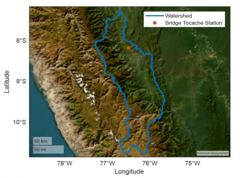
The 'Bridge Tocache' station is located in the lower part of the Upper Huallaga interbasin, one of the largest in Peru. Its coordinates are latitude -8.184750, longitude -76.507890, and altitude 479 meters above sea level. Flow data from the station exhibit significant seasonality influenced by the tropical climate, with peaks between January and March (e.g., 1,990.2 m³/s in March) and lows between June and August (e.g., 378.59 m³/s in August). This seasonal variability is crucial for understanding hydrological patterns and managing water resources effectively.
The Tocache station is located in the lower part of the interbasin, where flows from upstream areas converge, making it an ideal monitoring point as shown in Figure 1. This location provides representative and reliable measurements of the main channel, which are essential for hydrological studies and resource planning. The growing water demand in the interbasin further underscores the importance of this station. For instance, agricultural water permits increased from one in 1998 to 124 in 2018, while over 38% of households still lack access to potable water.
Figure 1. Location of the study station
2.2 Data preprocessing
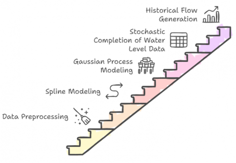
Data processing was performed using a workflow (Figure 2), to ensure the quality of the data used in the models, initial preprocessing was performed on both water level and flow data. During this stage, outliers or anomalous values that could compromise the accuracy of subsequent modeling were removed. The technique used for this purpose was percentiles, where appropriate thresholds were set to identify and remove values outside a reliable range. Previous studies have demonstrated the importance of removing these outliers to improve the accuracy of hydrological models, using similar approaches to ensure data representativeness [37].
Figure 2. Workflow
2.3 Model construction
Flow modeling was conducted based on water level information and month of the year, using two approaches:
Spline Model: A spline model was constructed to relate water levels with measured flows in the recent period (2020-2023). This model used only water level data as input and was adjusted using a parameter called adjustment factor. Splines allowed for precise modeling of nonlinear relationships and were well-suited for this type of problem [38]. The spline interpolation can be mathematically expressed as:
$S(x)=\sum_{i=1}^n a_i B_i(x)$ (1)
where, $S(x)$ is the spline function, $B_i(x)$ are the basis spline functions, and $a_i$ are the coefficients determined by the adjustment factor. The adjustment factor $\alpha$ controls the smoothness of the spline, balancing the trade-off between overfitting and underfitting the data.
Gaussian Process Model: A machine learning model based on Gaussian processes was implemented, which took water level data and the month of the year as inputs for the recent period (2020-2024). Including the month allowed the model to capture seasonal patterns and improve prediction accuracy. Gaussian processes were particularly useful for this type of problem due to their ability to estimate prediction uncertainty [39]. The Gaussian process can be defined by its mean function $m(x)$ and covariance function $k\left(x, x^{\prime}\right)$, such that:
$f(x) \sim G P\left(m(x), k\left(x, x^{\prime}\right)\right)$ (2)
where, $f(x)$ represents the flow prediction, $m(x)$ is typically assumed to be zero, and $k\left(x, x^{\prime}\right)$ is the kernel function that defines the covariance between any two input points $x$ and $x^{\prime}$.
2.4 Completion of missing water level data
Given that there were periods without recorded water level data, a stochastic process was applied to fill these gaps. To account for the hydrological variability and seasonal patterns of the region, the year was divided into 24 fortnights. This segmentation aligns with the bimodal rainfall distribution observed in the study area, allowing for more accurate modeling of water level fluctuations. Frequency distributions were then generated using kernel density estimation for each of these fortnights. With these distributions, random data were generated to follow the observed statistical behavior, allowing for the completion of missing periods. This process was repeated for all fortnights of the year, resulting in a continuous and consistent water level series [40].
2.5 Generation of the historical flow series
Once the water level data were completed and the flow prediction models adjusted, the historical flow series generation was carried out. The trained models were applied to estimate flows from 1997 to 2023. In this way, an extended and consistent database was obtained, which can be used for hydrological studies, model calibration, and infrastructure planning.
3.1 Data preprocessing
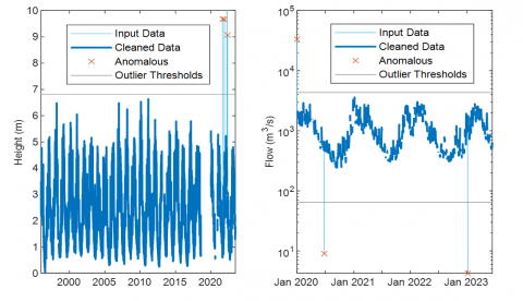
Data preprocessing is essential to ensure the quality of hydrological models. Four water level data points and three flow data points that were outside the acceptable ranges defined by the 0 and 99.95 percentiles for water level, and 0.2 and 99.83 percentiles for flow, were removed. This procedure filtered extreme values that could distort the results. These threshold values are consistent with those used in previous studies [41, 42], effectively distinguishing between spurious anomalies and significant hydrological events.
The use of percentiles to detect and remove outliers is a well-recognized methodology [34]. Previous studies have shown that higher percentiles improve accuracy in estimating extreme values in flow records, supporting this approach [34]. However, it is essential to ensure that the removed data do not represent rare but significant hydrological events. Alternative methods, such as modified Z-scores, provide additional options for outlier detection in water level data [43].
Figure 3. Data preprocessing
The methodology primarily relied on visual analysis to define the percentile thresholds, as shown in Figure 3. Although this method facilitates outlier identification, incorporating additional statistical techniques could enhance the objectivity of the process. Balancing the removal of outliers with the preservation of data reflecting legitimate extreme conditions is crucial, thus maintaining the integrity and representativeness of the data in modeling.
3.2 Modeling
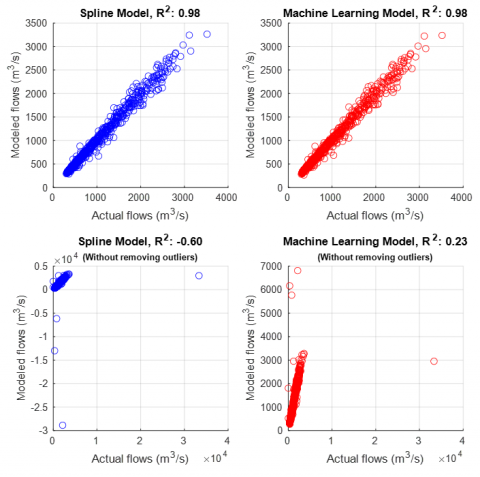
In this study, 590 pairs of water level or stage and flow data collected between January 2020 and June 2023 at the 'Bridge Tocache' station were analyzed. To model the relationship between water stage and flow, two main approaches were employed: a spline model and a model based on Gaussian processes. The spline model was developed using a smoothing factor of 0.85. Data points that deviated significantly from the general trend (i.e., those outside 3 standard deviations from the fitted line) were considered outliers and removed from the analysis, resulting in the exclusion of 8 data pairs (Figure 4). This approach is consistent with common practices in hydrological analysis, where removing outliers can improve model accuracy [43, 44]. The spline model achieved a coefficient of determination (R²) of 0.98, indicating an excellent fit to the observed data.
The effectiveness of splines in modeling nonlinear relationships in hydrological data has been highlighted in previous studies [45]. Splines provide greater flexibility in curve fitting, which is crucial for adequately representing the relationships between water stage and flow in rivers with changing characteristics. However, it is important to consider that outlier removal should be done cautiously. It is noted that excluding extreme values may lead to underestimating significant hydrological events, such as extreme floods, which are crucial for infrastructure design and risk management [46].
Figure 4. Spline data cleaning
The Gaussian process-based model incorporated water stage and month of the year as input variables in numerical format, allowing it to capture seasonal patterns and improve the model's robustness against temporal variations. The kernel hyperparameters were adjusted to optimize model performance, obtaining values of 0.8728, 18.9816, and 232.5542, while the sigma (noise) was 86.5131. The estimated beta coefficients (-227.3652, 661.1947, and -1.3325) reflect the influence of each variable on flow prediction. This model also achieved an R² of 0.98, demonstrating its high capacity to model flow variability.
3.3 Model sensitivity analysis to outliers and extreme events
Our analysis demonstrates that while outlier removal significantly enhances model performance, as evidenced by the high R² values (0.98) for both models, failing to remove outliers severely degrades the models' ability to predict rare events (see Figure 5). The spline model without outlier removal not only showed a poor R² of -0.60 but also exhibited inconsistent predictions, whereas the Gaussian process model, although more robust, still performed inadequately with an R² of 0.23. These findings underscore the importance of proper outlier management to ensure accurate prediction of critical hydrological events [47].
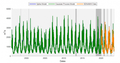
Figure 5. Performance of the spline and machine learning (Gaussian processes) models in flow prediction
The use of Gaussian processes in hydrology has gained attention due to their ability to handle uncertainties and model complex nonlinear relationships [48]. Gaussian process regression has been applied to monthly flow predictions, showing that this approach outperforms traditional models in accuracy and offers more reliable estimates [49]. Including seasonal variables, such as the month of the year, enhances the model’s ability to capture temporal patterns, which is essential in hydrological systems affected by climate cycles.
Both models in this study proved effective for predicting flows from historical water stage data, validating the approach used to generate an extended historical flow series at the 'Bridge Tocache' station. The high accuracy achieved with both methods suggests they can be applied in future hydrological model calibration studies and integrated water resource management in the Huallaga Basin.
The combination of spline-based models and Gaussian processes provides a robust tool to address the inherent complexity of hydrological systems. While splines offer flexibility in curve fitting and efficiently handle nonlinear relationships, Gaussian processes provide a probabilistic structure that allows for quantifying prediction uncertainty [42]. This dual approach aligns with recommendations to integrate different methodologies to improve understanding and prediction of hydrological processes [50]. For example, spline-based approaches have been effectively used to represent nonlinear runoff-generation mechanisms and capture abrupt changes in flow regimes. A notable case is the application of a B-spline quantile regression model at the Shigu station on the Jinsha River in China. This model processed daily runoff data and successfully generated predictive intervals with over 95% coverage, achieving grade-A accuracy with a deterministic coefficient (R²≥0.9). The model also constructed probability density functions that provided detailed insights into uncertainty and outperformed state-of-the-art methods in terms of robustness and computational efficiency [51]. Similarly, Gaussian process models have been employed to generate reliable predictive intervals for monthly streamflow forecasts. An application in five highly seasonal rivers in Ethiopia demonstrated their effectiveness in quantifying uncertainty under extreme climatic conditions, such as temperature increases up to 5℃ and precipitation variations of ±30%. These models provided consistent predictions and robust representations of uncertainty, even under data-scarce conditions, making them valuable tools for water resource management and climate change planning [52].
3.4 Stochastic completion of missing water level data
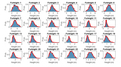
During the process of completing water level data, a total of 1,170 missing data points were identified for the period 1996-2023. The water level data presented a normal distribution with certain asymmetries in some fortnights of the year. Specifically, in some fortnights, water levels were lower compared to others, which may be due to the river's seasonality.
To address the missing data, kernel density estimation (KDE) distributions were used for each of the 24 fortnights of the year (see Figure 6). This approach allows estimating the probability density function of the data without assuming a specific parametric form, which is especially useful when the data exhibit asymmetries or multimodalities [53]. Applying KDE to each fortnight captures the specific characteristics and seasonality of the data during those periods.
Figure 6. Kernel density for height distributions
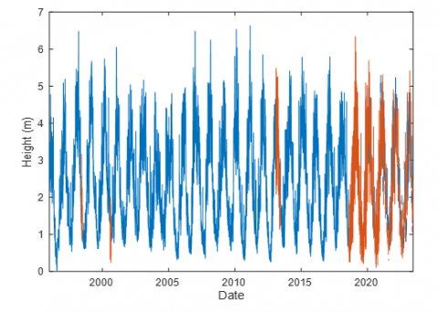
Figure 7 shows the stochastic completion of water level or stage data for the 'Bridge Tocache' river station. This stochastic imputation method aligns with recommended practices in hydrology, where imputation based on probabilistic methods may be more suitable than deterministic methods in cases with high seasonal variability [54].
However, it is important to consider the limitations of this approach. Stochastic imputation may introduce additional uncertainty into the completed data, and it is essential to evaluate the impact of these data on the developed models [55]. It must be ensured that the random data generation process does not violate the fundamental statistical properties of the original time series.
In similar studies, interpolation and imputation methods based on nearest neighbors have been used to fill missing data [56]. However, these methods may not adequately capture the seasonal variability, or asymmetries present in the data. The choice of KDE in this study reflects a careful consideration of the specific characteristics of the data and the need to preserve their statistical structure.
Figure 7, where the red lines represent the stochastically completed water levels, serves as a useful visual tool to assess the effectiveness of the imputation method and verify that the completed data integrate coherently with the observed data.
Figure 7. Height data completion
3.5 Flow generation
Table 1 compares the statistical characteristics of flows generated by two models-one based on splines and the other on machine learning-with actual flows, using a rank test to evaluate the similarity between distributions. The metrics analyzed include the mean, standard deviation, kurtosis, and skewness.
Table 1. Comparison of distribution metrics
|
Statistics |
p-valor |
|
|
Flow Spline |
Flow Machine Learning |
|
|
Average |
1 |
1 |
|
Standard Deviation |
1 |
1 |
|
Kurtosis |
0.99 |
0.99 |
|
Skewness |
0.98 |
0.99 |
The results obtained for each of these metrics are discussed below:
Mean: The p-values obtained for both comparisons (spline model-generated flows vs. actual flows and machine learning model-generated flows vs. actual flows) are equal to 1, indicating that there is no significant difference between the mean values of the modeled flows and the actual flows. This demonstrates that both models are capable of accurately reproducing the mean flow values (Figure 8), which is a key indicator of model quality in terms of overall accuracy. This result is consistent with previous studies that highlight the importance of capturing the mean in hydrological models to ensure reliable predictions [57].
Figure 8. Flow generation
Standard deviation: As with the mean, the p-values for the standard deviation are also 1 in both comparisons, suggesting that the variability or dispersion of the modeled flows does not differ significantly from that observed in the actual flows. Correctly capturing variability is essential in hydrological modeling, as it enables models to adequately reflect the natural dynamics and fluctuations of the system [58].
Kurtosis: The kurtosis values for both models (0.99) show a high similarity with actual flows in terms of the concentration of values around the mean. This implies that the models do not generate distributions that are either too flat or too peaked compared to the actual flow distribution. The ability of the models to replicate this metric is relevant in hydrological studies, as kurtosis affects the probability of extreme events, which are crucial for the design and management of water infrastructure [59].
Skewness: The skewness values obtained (0.98 for the spline model and 0.99 for the machine learning model) indicate that the distributions of flows generated by both models are nearly perfectly symmetrical compared to the actual distribution. The absence of a significant shift to the right or left suggests that the models do not introduce an artificial bias in the flow estimation, which is fundamental for the credibility and accuracy of the predictions [60].
p-value thresholds: In statistical analyses, p-values are commonly interpreted with a threshold of 0.05, indicating a 95% confidence level for rejecting the null hypothesis of no difference. In this context, p-values exceeding this threshold, such as those obtained in this study (all above 0.98), suggest a very high degree of similarity between the distributions of modeled and observed flows. In some cases, more stringent thresholds (e.g., 0.01) or less stringent ones (e.g., 0.10) are used depending on the requirements of the analysis. The choice of threshold should align with the study objectives, the implications of type I and type II errors, and the practical significance of the results. The p-values reported here reinforce the confidence in the models’ ability to replicate the statistical characteristics of observed flows accurately.
Overall interpretation: The statistical test results indicate that both models can replicate with high fidelity the fundamental statistical characteristics of the actual flows. This is significant because a good hydrological model must not only predict accurate mean values but also adequately represent the variability, shape, and symmetry of the data distribution [61]. The use of range tests to compare distributions is a standard practice in hydrological model validation, as it allows for assessing whether there are statistically significant differences between the modeled and observed distributions [62]. The fact that no significant differences were found in any of the metrics analyzed reinforces confidence in the predictive capability of the models used.
It is important to highlight that, although both models show similar performance in terms of the metrics analyzed, the choice between them may depend on other factors, such as computational complexity, interpretability, and data availability. Spline-based models are generally simpler and may be preferable in situations where simplicity and transparency are valued [63]. On the other hand, machine learning models, such as those based on Gaussian processes, may offer advantages in capturing more complex relationships and incorporating multiple predictor variables [42].
These results hold practical significance for hydrological applications. The similarity in statistical metrics (e.g., mean, standard deviation, skewness, and kurtosis) between the generated and observed flow series increases confidence in the reliability of the extended datasets. Such consistency suggests that the generated time series can be used with greater assurance in hydrological modeling, water resources planning, and risk assessment studies, where the availability of long-term flow data is crucial. Improved confidence in these metrics can support more informed decisions in infrastructure design, flood forecasting, and drought management, ultimately contributing to more robust and sustainable water management strategies.
The results of this study confirm the high performance of the proposed methodology for generating historical flow series from water level data using spline and Gaussian process models. Both approaches demonstrated excellent accuracy in reproducing observed flows, validating their reliability in contexts where flow data are scarce or unavailable. This performance highlights the flexibility and robustness of the models to capture nonlinear relationships, making them especially useful for various hydrological applications.
The potential of this methodology goes beyond its implementation in a single geographic location, as it can be adapted to different regions and river basins, provided water level records are available. Its capacity for generalization positions it as a versatile tool for water resource monitoring on a global scale. In particular, by integrating with low-cost hydrometric stations that only measure water levels, this methodology offers a viable and economical solution for countries with limited resources, enabling them to significantly improve the monitoring of their water bodies. A broader application of these models could facilitate a wider geographic coverage, strengthening the integrated management of water resources in contexts where access to advanced technology is limited.
Beyond monitoring, this methodology has additional practical applications, such as integration into early warning systems. By using the generated series to predict extreme flows, such as those associated with floods or droughts, it could contribute to disaster prevention and risk reduction. Furthermore, its flexibility allows for the incorporation of additional variables, opening possibilities for optimizing irrigation systems, estimating the discharge capacity of wastewater, or modeling hydraulic dynamics in more complex scenarios.
In the context of climate change, the methodology could be integrated into hydrological models that project future flow patterns. For example, extreme flows estimated from climate scenarios could be used inversely to determine associated water levels and evaluate the potential extent of flooding. This would be especially useful in planning resilient infrastructure and identifying areas vulnerable to overflows. Thus, the methodology not only addresses immediate monitoring needs but also provides tools to anticipate and mitigate the impacts of a changing climate, contributing to the sustainable development of water management policies.
[1] Sisay, E., Halefom, A., Khare, D., Singh, L., Worku, T. (2017). Hydrological modelling of ungauged urban watershed using SWAT model. Modeling Earth Systems and Environment, 3: 693-702. https://doi.org/10.1007/s40808-017-0328-6
[2] Liu, W., Park, S., Bailey, R.T., Molina-Navarro, E., Andersen, H.E., Thodsen, H., Nielsen, A., Jeppesen, E., Jensen, J.S., Jensen, J.B., Trolle, D. (2019). Comparing SWAT with SWAT-MODFLOW hydrological simulations when assessing the impacts of groundwater abstractions for irrigation and drinking water. Hydrology and Earth System Sciences Discussions, 2019: 1-51. https://doi.org/10.5194/HESS-2019-232
[3] Jeong, H.S., Seong, C.H., Park, S.W. (2014). Modeling daily streamflow in wastewater reused watersheds using system dynamics. Journal of The Korean Society of Agricultural Engineers, 56(6): 45-53. https://doi.org/10.5389/KSAE.2014.56.6.045
[4] Ahn, S.R., Jeong, J.H., Kim, S.J. (2016). Assessing drought threats to agricultural water supplies under climate change by combining the SWAT and MODSIM models for the Geum River basin, South Korea. Hydrological Sciences Journal, 61(15): 2740-2753. https://doi.org/10.1080/02626667.2015.1112905
[5] Madhushankha, J.M.L., Wijesekera, N.T.S. (2021). Application of HEC-HMS model to estimate daily streamflow in Badddegama Watershed of Gin Ganga Basin Sri Lanka. Engineer: Journal of the Institution of Engineers, Sri Lanka, 54(1): 89-97. https://doi.org/10.4038/engineer.v54i1.7438
[6] Matli C, Hunashal V. (2021). Hydrological modelling studies of Paravar river basin, a tributary of river Godavari using HEC-HMS model. Journal of Water Engineering and Management, 2(1): 48-54. https://doi.org/10.47884/jweam.v2i1pp48-54
[7] Liu, S., Shi, H., Niu, J., Chen, J., Kuang, X. (2020). Assessing future socioeconomic drought events under a changing climate over the Pearl River basin in South China. Journal of Hydrology: Regional Studies, 30: 100700. https://doi.org/10.1016/j.ejrh.2020.100700
[8] Byun, K., Hamlet, A.F. (2020). A risk-Based analytical framework for quantifying non-Stationary flood risks and establishing infrastructure design standards in a changing environment. Journal of Hydrology, 584: 124575. https://doi.org/10.1016/j.jhydrol.2020.124575
[9] Lu, D., Tighe, S.L., Xie, W.C. (2018). Pavement risk assessment for future extreme precipitation events under climate change. Transportation Research Record, 2672(40): 122-131. https://doi.org/10.1177/0361198118781657
[10] Sirisena, T.J.G., Maskey, S., Ranasinghe, R. (2020). Hydrological model calibration with streamflow and remote sensing based evapotranspiration data in a data poor basin. Remote Sensing, 12(22): 3768. https://doi.org/10.3390/rs12223768
[11] Lee, J.S., Choi, H.I. (2021). Improved streamflow calibration of a land surface model by the choice of objective functions-A case study of the Nakdong river watershed in the Korean peninsula. Water, 13(12): 1709. https://doi.org/10.3390/w13121709
[12] Feyen, L., Kalas, M., Vrugt, J.A. (2008). Semi-Distributed parameter optimization and uncertainty assessment for large-Scale streamflow simulation using global optimization/Optimisation de paramètres semi-Distribués et évaluation de l'incertitude pour la simulation de débits à grande échelle par l'utilisation d'une optimisation globale. Hydrological Sciences Journal, 53(2): 293-308. https://doi.org/10.1623/hysj.53.2.293
[13] De Lavenne, A., Thirel, G., Andréassian, V., Perrin, C., Ramos, M.H. (2016). Spatial variability of the parameters of a semi-Distributed hydrological model. Proceedings of the International Association of Hydrological Sciences, 373: 87-94. https://doi.org/10.5194/PIAHS-373-87-2016
[14] Lu, M., Lall, U., Robertson, A.W., Cook, E. (2017). Optimizing multiple reliable forward contracts for reservoir allocation using multitime scale streamflow forecasts. Water Resources Research, 53(3): 2035-2050. https://doi.org/10.1002/2016WR019552
[15] Yassin, F., Razavi, S., Elshamy, M., Davison, B., Sapriza-Azuri, G., Wheater, H. (2019). Representation and improved parameterization of reservoir operation in hydrological and land-surface models. Hydrology and Earth System Sciences, 23(9): 3735-3764. https://doi.org/10.5194/hess-23-3735-2019
[16] Ly, K., Metternicht, G., Marshall, L. (2020). Simulation of streamflow and instream loads of total suspended solids and nitrate in a large transboundary river basin using Source model and geospatial analysis. Science of the Total Environment, 744: 140656. https://doi.org/10.1016/j.scitotenv.2020.140656
[17] Li, X., Yang, X., Gao, W. (2006). An integrative hydrological, ecological and economical (HEE) modeling system for assessing water resources and ecosystem production: Calibration and validation in the upper and middle parts of the Yellow River Basin, China. In Proceedings Volume 6298, Remote Sensing and Modeling of Ecosystems for Sustainability III, San Diego, California, United States, p. 62982I-1. https://doi.org/10.1117/12.680713
[18] Kim, Y.W., Lee, J.W., Woo, S.Y., Lee, J.J., Hur, J.W., Kim, S.J. (2023). Design of ecological flow (E-Flow) considering watershed status using watershed and physical habitat models. Water, 15(18): 3267. https://doi.org/10.3390/w15183267
[19] Parker, S.R., Adams, S.K., Lammers, R.W., Stein, E.D., Bledsoe, B.P. (2019). Targeted hydrologic model calibration to improve prediction of ecologically-relevant flow metrics. Journal of Hydrology, 573: 546-556. https://doi.org/10.1016/j.jhydrol.2019.03.081
[20] Tendall, D.M., Hellweg, S., Pfister, S., Huijbregts, M.A., Gaillard, G. (2014). Impacts of river water consumption on aquatic biodiversity in life cycle assessment-A proposed method, and a case study for Europe. Environmental Science & Technology, 48(6): 3236-3244. https://doi.org/10.1021/es4048686
[21] Shah, R.D.T., Sharma, S., Bharati, L. (2020). Water diversion induced changes in aquatic biodiversity in monsoon-dominated rivers of Western Himalayas in Nepal: Implications for environmental flows. Ecological Indicators, 108: 105735. https://doi.org/10.1016/j.ecolind.2019.105735
[22] Lozano, D., Mateos, L., Merkley, G.P., Clemmens, A.J. (2009). Field calibration of submerged sluice gates in irrigation canals. Journal of Irrigation and Drainage Engineering, 135(6): 763-772. https://doi.org/10.1061/(ASCE)IR.1943-4774.0000085
[23] Spruill, C.A., Workman, S.R., Taraba, J.L. (2000). Simulation of daily and monthly stream discharge from small watersheds using the SWAT model. Transactions of the ASAE, 43(6): 1431-1439. https://doi.org/10.13031/2013.3041
[24] Radinja, M., Comas, J., Corominas, L., Atanasova, N. (2019). Assessing stormwater control measures using modelling and a multi-Criteria approach. Journal of Environmental Management, 243: 257-268. https://doi.org/10.1016/j.jenvman.2019.04.102
[25] Shiau, J.T., Shen, H.W. (2001). Recurrence analysis of hydrologic droughts of differing severity. Journal of Water Resources Planning and Management, 127(1): 30-40. https://doi.org/10.1061/(ASCE)0733-9496(2001)127:1(30)
[26] Cancelliere, A., Salas, J.D. (2010). Drought probabilities and return period for annual streamflows series. Journal of Hydrology, 391(1-2): 77-89. https://doi.org/10.1016/J.JHYDROL.2010.07.008
[27] Wi, S., Yang, Y.C.E., Steinschneider, S., Khalil, A., Brown, C.M. (2015). Calibration approaches for distributed hydrologic models in poorly gaged basins: Implication for streamflow projections under climate change. Hydrology and Earth System Sciences, 19(2): 857-876. https://doi.org/10.5194/HESS-19-857-2015
[28] Smith, K.A., Barker, L.J., Tanguy, M., Parry, S., Harrigan, S., Legg, T.P., Prudhomme, C., Hannaford, J. (2019). A multi-Objective ensemble approach to hydrological modelling in the UK: An application to historic drought reconstruction. Hydrology and Earth System Sciences, 23(8): 3247-3268. https://doi.org/10.5194/HESS-23-3247-2019
[29] Bjerklie, D.M., Birkett, C.M., Jones, J.W., Carabajal, C., Rover, J.A., Fulton, J.W., Garambois, P.A. (2018). Satellite remote sensing estimation of river discharge: Application to the Yukon River Alaska. Journal of Hydrology, 561: 1000-1018. https://doi.org/10.1016/j.jhydrol.2018.04.005
[30] Jachens, E.R., Roques, C., Rupp, D.E., Selker, J.S. (2020). Streamflow recession analysis using water height. Water Resources Research, 56(6): e2020WR027091. https://doi.org/10.1029/2020WR027091
[31] Maghrebi, M.F., Vatanchi, S.M., Kawanisi, K. (2023). Investigation of stage‐Discharge model performance for streamflow estimating: A case study of the Gono River, Japan. River Research and Applications, 39(5): 805-818. https://doi.org/10.1002/rra.4106
[32] Jin, L.S., Ha, H.M., Sung, L.B., Hwan, K.I. (2006). Development of a stream discharge estimation program. Journal of the Korean Society of Agricultural Engineers, 48(1): 27-38. https://doi.org/10.5389/KSAE.2006.48.1.027
[33] Birkinshaw, S.J., O'donnell, G.M., Moore, P., Kilsby, C.G., Fowler, H.J., Berry, P.A.M. (2010). Using satellite altimetry data to augment flow estimation techniques on the Mekong River. Hydrological Processes, 24(26): 3811-3825. https://doi.org/10.1002/hyp.7811
[34] Li, G., Wei, Y., Chi, Y., Chen, Y. (2024). A sharp convergence theory for the probability flow odes of diffusion models. arXiv Preprint arXiv: 2408.02320. https://doi.org/10.48550/arXiv.2408.02320
[35] Cheng, C., Li, J., Peng, J., Liu, G. (2024). Categorical flow matching on statistical manifolds. arXiv Preprint arXiv: 2405.16441. https://doi.org/10.48550/arXiv.2405.16441
[36] Boll, B., Gonzalez-Alvarado, D., Petra, S., Schnörr, C. (2024). Generative assignment flows for representing and learning joint distributions of discrete data. arXiv Preprint arXiv: 2406.04527. https://doi.org/10.48550/arXiv.2406.04527
[37] Nalley, D., Adamowski, J., Khalil, B., Biswas, A. (2020). A comparison of conventional and wavelet transform based methods for streamflow record extension. Journal of Hydrology, 582: 124503. https://doi.org/10.1016/j.jhydrol.2019.124503
[38] Knight, J.H., Rassam, D.W. (2007). Groundwater head responses due to random stream stage fluctuations using basis splines. Water Resources Research, 43(6). https://doi.org/10.1029/2006WR005155
[39] Yuan, L., Forshay, K.J. (2021). Enhanced streamflow prediction with SWAT using support vector regression for spatial calibration: A case study in the Illinois River watershed, US. PLoS One, 16(4): e0248489. https://doi.org/10.1371/journal.pone.0248489
[40] Sharma, A., Tarboton, D.G., Lall, U. (1997). Streamflow simulation: A nonparametric approach. Water Resources Research, 33(2): 291-308. https://doi.org/10.1029/96WR02839
[41] Sarailidis, G., Vasiliades, L., Loukas, A. (2019). Analysis of streamflow droughts using fixed and variable thresholds. Hydrological Processes, 33(3): 414-431. https://doi.org/10.1002/hyp.13336
[42] Giuntoli, I., Vidal, J.P., Prudhomme, C., Hannah, D.M. (2015). Future hydrological extremes: The uncertainty from multiple global climate and global hydrological models. Earth System Dynamics, 6(1): 267-285. https://doi.org/10.5194/esd-6-267-2015
[43] Bae, I., Ji, U. (2019). Outlier detection and smoothing process for water level data measured by ultrasonic sensor in stream flows. Water, 11(5): 951. https://doi.org/10.3390/W11050951
[44] Gotway, C.A. (1994). Statistical methods in water resources. Technometrics, 36(3): 323-324. https://doi.org/10.1080/00401706.1994.10485818
[45] Turpin, K.M., Lapen, D.R., Gregorich, E.G., Topp, G.C., McLaughlin, N.B., Curnoe, W.E., Robin, M.J.L. (2003). Application of multivariate adaptive regression splines (MARS) in precision agriculture. In Precision Agriculture. Wageningen Academic, pp. 677-682. https://doi.org/10.3920/9789086865147_104
[46] Klemeš, V. (1986). Operational testing of hydrological simulation models. Hydrological Sciences Journal, 31(1): 13-24. https://doi.org/10.1080/02626668609491024
[47] Boldetti, G., Riffard, M., Andréassian, V., Oudin, L. (2010). Data-Set cleansing practices and hydrological regionalization: is there any valuable information among outliers? Hydrological Sciences Journal-Journal des Sciences Hydrologiques, 55(6): 941-951. https://doi.org/10.1080/02626667.2010.505171
[48] Rasmussen, C.E. (2003). Gaussian processes in machine learning. In Summer School on Machine Learning. Springer, Berlin, Heidelberg, pp. 63-71. https://doi.org/10.1007/978-3-540-28650-9_4
[49] Sun, A.Y., Wang, D., Xu, X. (2014). Monthly streamflow forecasting using Gaussian process regression. Journal of Hydrology, 511: 72-81. https://doi.org/10.1016/j.jhydrol.2014.01.023
[50] Wheater, H.S., Jakeman, A.J., Beven, K.J. (1993). Progress and directions in rainfall-runoff modelling. Modelling Change in Environmental Systems, 101-132. https://acortar.link/loVWnr.
[51] He, Y., Fan, H., Lei, X., Wan, J. (2021). A runoff probability density prediction method based on B-Spline quantile regression and kernel density estimation. Applied Mathematical Modelling, 93: 852-867. https://doi.org/10.1016/J.APM.2020.12.043
[52] Shortridge, J.E., Guikema, S.D., Zaitchik, B.F. (2016). Machine learning methods for empirical streamflow simulation: A comparison of model accuracy, interpretability, and uncertainty in seasonal watersheds. Hydrology and Earth System Sciences, 20(7): 2611-2628. https://doi.org/10.5194/HESS-20-2611-2016
[53] Silverman, B.W. (2018). Density Estimation for Statistics and Data Analysis. Routledge, New York. https://doi.org/10.1201/9781315140919
[54] Little, R.J., Rubin, D.B. (2019). Statistical Analysis with Missing Data. John Wiley & Sons. http://doi.org/10.1002/9781119482260
[55] Schafer, J.L., Graham, J.W. (2002). Missing data: Our view of the state of the art. Psychological Methods, 7(2): 147-177. https://doi.org/10.1037/1082-989X.7.2.147
[56] Fatichi, S., Rimkus, S., Burlando, P., Bordoy, R. (2014). Does internal climate variability overwhelm climate change signals in streamflow? The upper Po and Rhone basin case studies. Science of the Total Environment, 493: 1171-1182. https://doi.org/10.1016/j.scitotenv.2013.12.014
[57] Moriasi, D.N., Arnold, J.G., Van Liew, M.W., Bingner, R.L., Harmel, R.D., Veith, T.L. (2007). Model evaluation guidelines for systematic quantification of accuracy in watershed simulations. Transactions of the ASABE, 50(3): 885-900. https://doi.org/10.13031/2013.23153
[58] Gupta, H.V., Kling, H., Yilmaz, K.K., Martinez, G.F. (2009). Decomposition of the mean squared error and NSE performance criteria: Implications for improving hydrological modelling. Journal of Hydrology, 377(1-2): 80-91. https://doi.org/10.1016/j.jhydrol.2009.08.003
[59] Hosking, J.R.M., Wallis, J.R. (1997). Regional Frequency Analysis: An Approach Based on L-Moments. Cambridge University Press. https://doi.org/10.1017/CBO9780511529443
[60] Beven, K.J. (2012). Rainfall-Runoff Modelling: The Primer. John Wiley & Sons. https://doi.org/10.1002/9781119951001
[61] Dawson, C.W., Wilby, R.L. (2001). Hydrological modelling using artificial neural networks. Progress in Physical Geography, 25(1): 80-108. https://doi.org/10.1177/030913330102500104
[62] Zhang, X., Srinivasan, R., Hao, F. (2007). Predicting hydrologic response to climate change in the Luohe River basin using the SWAT model. Transactions of the ASABE, 50(3): 901-910. https://doi.org/10.13031/2013.23154
[63] Shrestha, D.L., Solomatine, D.P. (2006). Machine learning approaches for estimation of prediction interval for the model output. Neural Networks, 19(2): 225-235. https://doi.org/10.1016/j.neunet.2006.01.012