Oubaida Masadeh*![]() | Esraa Radi Tarawneh
| Esraa Radi Tarawneh![]()
© 2025 The authors. This article is published by IIETA and is licensed under the CC BY 4.0 license (http://creativecommons.org/licenses/by/4.0/).
OPEN ACCESS
Climate change is anticipated to alter precipitation patterns, which could lead to in increased frequency and severity of flooding events that threaten populations and infrastructure. Comprehending these effects is crucial for enhancing flood management measures. This research employs the hydrologic engineering center's hydrologic modeling system (HEC-HMS) in conjunction with future climate forecasts to evaluate flood hazards in Jordan's Wadi Al Mujib Basin. Climate forecasts utilize the most recent global climate models from the coupled model intercomparison project phase 6 (CMIP6), which offers different future scenarios relates to greenhouse gas emissions, known as shared socioeconomic pathways (SSPs). Four scenarios’ data for study area were employed: SSP126 (low emissions), SSP245 (moderate emissions), SSP370 (high emissions), and SSP585 (extremely high emissions). Results indicate that higher-emission scenarios (SSP370 and SSP585) lead to a significant increase in rainfall intensity and flood frequency, especially for extended storm duration and longer return periods. Peak discharge values are closely following rainfall trends, with minimal differences between observed and projected floods for the 2- and 5-year return periods under SSP245 and SSP370. However, under SSP370 and particularly SSP585, peak discharge increases substantially for the 50- and 100-year return periods, highlighting the increased risk of floods caused by increased emissions. These findings underline the importance of integrating hydrological models with climate projections for forecasting flood dangers. This methodology can assist policymakers and engineers to develop adaptable flood mitigation strategies that reduce the escalating hazards associated with climate change.
climate change, CMIP6, SSPs, hydrological modeling, flood
Climate change has changed the number and severity of flooding events worldwide [1], causing many problems for communities, especially in arid regions [2]. Jordan has desert climate [3]. Jordan's low greenhouse gas (GHG) emissions make it a negligible contributor to global climate change [4], but climate-related disasters like flash floods, landslides, rock falls, and droughts have killed 110 people, affected hundreds of thousands, and caused significant economic losses over the past 30 years [5]. Thus, successful disaster management and mitigation require accurate flood risk estimation based on flood-frequency analysis, which uses past rainfall and flood data to predict future flood magnitude and recurrence [6].
Current population trends show that global urbanisation has major direct and indirect effects on climate and weather. Under global climate change and variability, extreme events are more likely. Floods, unpredictability in rainfall patterns, and heat wave variability may be caused by climate change [7], which may affect dam design and operation. Thus, these changes affect hydropower and water supply. Thus, accurate identification of how climate change affects flood events is essential for drought risk management and flood control [8].
Hydrological modelling helps understand and predict climate change's effects on flood events by simulating diverse hydrological processes in changing climates [9]. Research objectives, data, and watershed attributes determine hydrological model selection [10]. The hydrologic engineering center's hydrologic modeling system (HEC-HMS) model has been widely used to model rainfall-runoff processes to assess how climate change affects flood behaviour [11]. Using HEC-HMS to assess flood risk in the Bagmati river basin in Nepal, high-emission scenarios increased peak flow, resulting in rainfall-runoff correlations and a flood discharge modelling tool [12]. Using the HEC-HMS model, the study [13] predicted climate-induced streamflow variability in the Blue Nile Basin. Another SWAT model study examined how climate change affects streamflow in the Mesoscale Rur watershed in western Germany, highlighting the risk of floods under higher precipitation levels [14].
HEC-HMS, designed by the U.S. Army Corps of Engineers, is widely used to simulate watershed-scale hydrological processes and evaluate flood dynamics [15]. HEC-HMS has been a versatile tool for climate change impact assessments, watershed management, and flood forecasting worldwide since its founding [16]. It can model precipitation-runoff relationships, channel flow, and flood hydrographs for many hydrological conditions and regions [17]. Users can evaluate storms and land-use changes using the model's basin modelling, meteorological modelling, control specifications, and simulation results analysis [11]. By calibrating and validating simulated outputs with real data, HEC-HMS improves flood risk assessment and water resource planning [18].
HEC-HMS has been used worldwide to model hydrological processes, flood risks, and runoff [19]. Al-Mukhtar and Al-Yaseen [20] simulated peak discharge and volumes for the Ngong River basin in Nairobi utilising HEC-HMS. The study [21] applied the model to evaluate flood management measures in the Audi-União District in Brazil. HEC-HMS also assessed how land-use changes affected the Kan watershed in Tahran, Iran [22].
Due to climate projection uncertainty, several models have been developed to guide hydrological events under climate change [23]. The coupled model intercomparison project (CMIP) has progressed through several phases to improve climate knowledge [24]. CMIP Phase 6 (CMIP6) presents an updated set of scenarios called shared socioeconomic pathways (SSPs) [25], which improve on Representative Concentration Pathways (RCPs) from CMIP5 [26]. By varying radiative forcing (2.6-8.5 W/m² by 2100), RCPs were used to study potential greenhouse gas emission pathways [27]. The more integrated SSP approach combines socioeconomic factors with RCP-style radiative forcing levels [28]. This allows for more advanced climate change research, especially on hydrological extremes like floods [29]. SSPs allow researchers to assess climate change's wider effects under different emission and adaptation scenarios by including economic development and policy reactions [30].
This research employed four SSPs-SSP126, 245, 370, and SSP585- to evaluate prospective flood hazards in the Wadi Al Mujib Basin. These scenarios were selected to examine a wide range of possible climate circumstances, from a low-emission, sustainability-oriented future (SSP126) to a high emission, worst case scenario (SSP585). Although previous research has investigated the effects of climate change on flooding using RCPs, there is a lack of studies that combine HEC-HMS hydrological modeling with CMIP6 SSPs in arid and semi-arid areas such as Wadi Al Mujib. This work addresses the gap by delivering more sophisticated prospective flood hazards, providing valuable insights for adaptive flood management and policy formulation in Jordan.
The Al Mujib Basin, an essential water resource in Jordan, covers an area of 6,456 km², or around 7.22% of Jordan’s land area. The area falls into two sub-catchments: Wadi Al Mujib (4,419 km²) and Wadi Al Walaa (2,037 km²). The area falls into two sub-catchments: Wadi Al Mujib (4,419 km²) and Wadi Al Walaa (2,037 km²). The basin spans four governorates: Madaba (6.01%) and Amman (35.13%) in the center region, and Karak (33.09%) and Ma'an (25.77%) in the southern region. The basin serves as crucial for supply of water, agriculture, and groundwater recharge.
The basin exhibits an extensive variety of elevations and gradients. Most of the basin lies between 667 and 1269 meters above sea level, with a small portion falling below sea level. Consequently, it influences runoff dynamics and hydrological responses (Figure 1).
Figure 1. Al Mujib Basin features (slope, location and elevation) and gauges locations (rainfall and discharge stations)
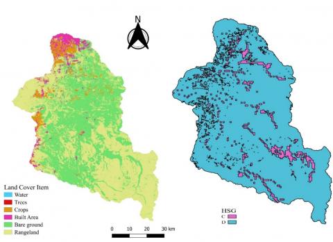
For essential HEC-HMS data, discharge station data from CD0041, located at the basin outlet, which recorded observations from 1980 to 1998 and was utilized in model calibration. On the other side, Water and Irrigation Ministry of Jordan's rainfall stations data from 1980 to 2023 was used as the main source of precipitation data to construct the hydrological model. in addition, land cover and land use (LCLU) data for 2021 was acquired by analyzing Sentinel-2 satellite images at a 10-meter resolution. As well, soil properties were derived from the Global Hydrologic Soil Groups (HYSOGs250m) dataset, which belongs to Oak Ridge National Laboratory Distributed Active Archive Center (ORNL DAAC). Figure 2 presents the spatial distribution of LCLU and Hydrologic Soil Groups (HSGs) across the basin. Table 1 shows the information of precipitation gauges.
Figure 2. Al Mujib Basin LCLU and HSG
Table 1. Information of precipitation gauges
|
Station ID |
Station Name |
Palestine North (km) |
Palestine East (km) |
Latitude |
Longitude |
Elevation (m) |
|
CD0006 |
WADI WALA EVAP. ST |
1107500 |
223000 |
31.56 |
35.77 |
494 |
|
CD0010 |
RABBA EVAP.ST |
1075500 |
220500 |
31.27 |
35.74 |
965 |
|
CD0020 |
SIWAQA EVAP ST. |
1086800 |
253700 |
31.37 |
36.09 |
731 |
|
CD0003 |
EL MUWAQQAR |
1136500 |
255000 |
31.82 |
36.11 |
907 |
|
CD0016 |
JUDAYDA |
1105000 |
211500 |
31.54 |
35.65 |
770 |
|
CD0001 |
SAHAB |
1142500 |
245000 |
31.87 |
36.00 |
860 |
|
CD0007 |
DHIBAN |
1100800 |
224000 |
31.50 |
35.78 |
720 |
|
CD0011 |
QATRANA POLICE POST |
1072500 |
249500 |
31.24 |
36.04 |
771 |
|
CD0023 |
QASR EVAP. ST |
1080900 |
221000 |
31.32 |
35.75 |
721 |
|
CC0004 |
MUSHAQQAR EVAP. ST |
1132900 |
22620 |
31.79 |
35.80 |
841 |
3.1 Model setup
HEC-HMS Version 4.12 was employed to simulate rainfall-runoff dynamics in the Wadi Al Mujib Basin. The model consists of a basin model that depicts watershed characteristics, a meteorological model for climatic inputs, and control specifications for establishing simulation parameters. The model development began with the import of a 30-meter Digital Elevation Model (DEM) to delineate sub-basins and extract hydrologically relevant features using the Sink Fill method.
Thirty-one sub-basins and fourteen reaches were identified (Figure 3). Curve Number (CN), land use, soil cover, and antecedent moisture conditions were derived by using spatially distributed LCLU and HSG data. The CN method (Figure 3) was employed for rainfall-runoff transformation to ensure the model captured spatial and temporal variations in infiltration and runoff generation. Precipitation input was based on historical rainfall data (1980-2023) stations. However, areal precipitation was computed by assigning representative weights to each gauge by using the Thiessen polygon.
Figure 3. Curve number and impervious percentage for each subbasin, reaches, discharge and rainfall stations
Muskingum method, for flow routing, was selected due to its suitability for channel storage representation in the basin. Whilst Clark Unit Hydrograph method was used for runoff transformation, and for reflect the watershed response dynamics concentration time (Tc) and storage coefficient (R) were incorporated.
Tc and R in relation to precipitation and watershed properties are:
${{T}_{c}}=2.2\times {{(\frac{L*{{L}_{c}}}{\sqrt{Slop{{e}_{{{10}^{-85}}}}}})}^{0.3}}$ (1)
$\frac{R}{{{T}_{c}}+R}=0.65$ or$\text{ }\!\!~\!\!\text{ }\!\!~\!\!\text{ }R=\frac{13}{7}{{T}_{c}}$ (2)
These parameters were determined based on watershed characteristics, where L denotes the longest flow path mile, $L_c~$ is the centroidal flow path in mile and slope 10-85 is average slope of the flow path represented by 10 to 85 percent of the longest flow path (ft/mi) [31, 32].
3.2 Model calibration and validation
March 1991 and January 1998 floods were among the most notable in the seven-year streamflow statistics at Wadi Al Mujib Basin station CD0041. Several factors led to the selection of these events for HEC-HMS model calibration and validation. First, this period's minimal land use and land cover changes-maintained watershed characteristics. The short time between these events reduced the likelihood of significant changes in other watershed attributes like soil properties or basin slope. The March 1991 event was used for model calibration. Parameters influencing hydrological processes, such as the CN in the SCS method, time of concentration (Tc), and storage coefficient (R) in the Clark Unit Hydrograph method, were adjusted to ensure the simulated discharge accurately corresponded with the observed data regarding of peak discharge, hydrograph shape, and timing of the peak. Calibration trials employed the Peak-Weighted RMS Error objective function with the Univariate Gradient method to minimize discrepancies systematically. The Nash-Sutcliffe efficiency coefficient (E) was used to evaluate the model's performance quantitatively is shown in:
$E=1-\frac{\mathop{\sum }_{i=1}^{n}{{\left( {{Q}_{o,i}}-{{Q}_{s,i}} \right)}^{2}}}{\mathop{\sum }_{i=1}^{n}{{\left( {{Q}_{o,i}}-\overline{{{Q}_{o}}} \right)}^{2}}}$ (3)
where, ${{Q}_{o,i}}$ denotes observed discharge at time step i, ${{Q}_{s,i}}$ is the simulated discharge at time step i,$~\overline{{{Q}_{o}}}$ is mean of the observed discharges and n is the total number of time steps.
Nash-Sutcliffe efficiency coefficient ranges from -∞ to 1, when it equal is one, that means simulated and observed peak discharge perfectly match, but when its value is zero this implies model predictions are as mean of the observed data. Whereas negative values indicate that the observed mean is better than model [33].
A wide range of general circulation model (GCM) eeriments have been to investigate the anticipated climatic consequences of rising greenhouse gas emissions [34]. The CMIP has created global climate projection datasets using standardised experimental protocols. However, GCMs have much lower spatial resolution than hydrological modelling at wshed or sub-watershed scales [35], usually hundreds to tusands of kilometres. Due to this scale mismatch, downscaling techniques are needed to bridge the gap between global climate models and localised hydrological assessments [35]. Regional climate models (RCMs) and statistical or dynamical downscaling methods [36] refine the coarse outputs of global models to generate detailed climate data tailored to hydrologic studies. Coordinated Regional Climate Downscaling Experiment (CORDEX) is used to evaluate RCMs and downscaling methods [37]. By providing uniform regional simulation methods, CORDEX helps evaluate model accuracy and generates high-resolution climate data for impact assessments. This framework also helps connect local environmental studies with global climate scenarios from the RCPs and SSPs to analyse regional climate impacts [38]. In this study, high-resolution climate projection data from the Max Planck Institute for Meteorology’s MPI-ESM1-2-HR model was utilized. As a key partner in the CMIP6 HighResMIP project, this model provided both historical flux precipitation data for this study from 1900-2014 and future projections under different climate scenarios from 2015-2100. The data encompasses various SSPs including SSP126, 245, 370, and SSP585, and using particular equations provided below, the statistical downscaling technique known as linear scaling bias correction, which guarantees that the corrected climate projections more closely match observed historical values, this technique seeks to minimize the inherent biases in regional climate model simulations by means of more precise inputs for hydrological climate-change impact studies.
${{p}^{*}}_{Contr}\left( d \right)={{P}_{Contr}}\left( d \right).\left[ \frac{{{\mu }_{m}}\left( {{p}_{obs}}\left( d \right) \right)}{{{\mu }_{m}}\left( {{P}_{contr}}\left( d \right) \right)} \right]$ (4)
${{p}^{*}}_{scen}\left( d \right)={{P}_{scen}}\left( d \right).\left[ \frac{{{\mu }_{m}}\left( {{p}_{obs}}\left( d \right) \right)}{{{\mu }_{m}}\left( {{p}_{contr}}\left( d \right) \right)} \right]$ (5)
where, ${{P}_{Contr}}\left( d \right)$ donates precipitation of control scenario (day), ${{P}_{scen}}\left( d \right)$ is the precipitation of scenario (day), ${{p}^{*}}_{Contr}~$ is the adjusted precipitation of control scenario for (day), ${{p}^{*}}_{scen}\left( d \right)$ is the adjusted precipitation of scenario for (day), ${{\mu }_{m}}\left( {{p}_{obs}}\left( d \right) \right)$ is the mean observed precipitation for (day) and ${{\mu }_{m}}\left( {{p}_{contr}}\left( d \right) \right)$ is the mean precipitation of control scenario for (day).
Linear scaling method accurately adjusts mean precipitation data, but it has limits, especially in capturing extreme precipitation events, which are vital for flood modeling. Linear scaling assumes that biases stay the same for all levels of precipitation. This could lead to the underestimation of infrequent events crucial for peak discharge in hydrological models. Conversely, alternative techniques like quantile mapping offer a more precise adjustment for severe occurrences but require comprehensive observational datasets to obtain accurate distributions.
MPI-ESM1-2-HR model was chosen for its improved spatial resolution and proven efficacy in modeling precipitation and temperature variations in arid and semi-arid areas. In comparison to other CMIP6 models, such as GFDL-ESM4 or CESM2, MPI-ESM1-2-HR has a higher spatial resolution (about 100 km) and has been widely utilized in regional climate impact studies, making it an appropriate selection for evaluating climate change effects in the Wadi Al Mujib Basin.
Figure 4. Overview of SSPs and their challenges for mitigation and adaptation [39]
As illustrated in Figure 4, the SSPs include SSP1-2.6 (sustainable development, low emissions), SSP2-4.5 (middle-of-the-road development, moderate emissions), SSP3-7.0 (regional rivalry, high emissions), and SSP5-8.5 (fossil-fueled development, very high emissions). These pathways are invaluable for generating time-dependent projections of greenhouse gas emissions, radiative forcing, and their impacts, aiding in both mitigation strategy assessment and climate risk analysis [40]. In this study, SSP1-2.6, 2-4.5, 3-7.0, and SSP5-8.5 are used to represent low, moderate, high, and very high greenhouse gas emission scenarios, respectively.
5.1 LCLU and HSG
LCLU classifies the scene as desolate. The Wadi Al Mujib Basin was 94% bare ground, 3% built-up, and 2% agricultural. This indicates little farming. The remaining 1% includes trees, water, and land uses. This distribution shows the basin's arid and semi-arid climate, which limits vegetation and agriculture. Group D soils with high runoff potential and low infiltration cer most of the basin, according to the HSG study. The basin's hydrological response and flooding susceptibility are affected by sparse land cover, heavy rainfall, and surface roff, wch generate and strengthen floods.
En though Wadi al Mujib doesn't have a lot of developed land, human activities like building cities, improving infrastructure, and changing the way farms work are changing the way water flows through the basin. Meanwhile, the expansion of impervious surfaces like roads will likely reduce infiltration while increasing runoff, therefore aggravating flood risks. Additionally, agricultural practices, although limited in the study area, may contribute to soil degradation and reduced water retention capacity.
5.2 Projection and observed precipitation
Cibrated precipitation data from 1900 to 2014 was used as the control scenario for comparison. In the calibration phase, lear scaling and bias correction reduced differences between simulated and observed precipitation data, improving the baseline model's accuracy. The calibrated model projected 2015-2100 precipitation trends under several SSPs.
In Figure 5, the Wadi Al Mujib Basin's precipitation frequencies for different return intervals and durations show clear patterns. The 100-year return period precipitation amounts for 1, 2, 3, 4, and 5 days are 53.15 mm, 90.88 mm, 112.91 mm, 121.94 mm, and 127.90 mm. The fifth day of 100-year precipitation is 15.96 mm (13%), while the fifth day of 50-year precipitation is 7.48 mm (7%). These findings show that precipitation intensities increase with duration, but over longer periods, the difference between durations becomes irrelevant. Data shows that most of the 5-day precipitation occurs in the first few days due to their higher quantities, but they are not significantly different from shorter periods.
Figure 5. Observed precipitation in Al Mujib Basin
Figures 6-9 show that precipitation intensities rise with longer return times and durations for the selected SSPs. In the SSP126 scenario Figure 6, 100-year precipitation values for 1, 2, 3, 4, and 5 days are 73.72, 108.78, 125.34, 135.29, and 141.78 mm. The 5-day 100-year precipitation is 4.8% higher than the 4-day. In Figure 7, SSP 245 precipitation amounts to 86.13, 122.8, 142.77, 152.35, and 160.26 mm. The 100-year precipitation values for 1, 2, 3, 4, and 5 days in the SSP370 scenario Figure 8 are 78.10, 110.47, 136.03, 152.17, and 162.11 mm. The 5-day precipitation is 6.5% higher than the 4-day. The SSP585 scenario (Figure 9) predicts 90.74, 133.20, 156.68, 165.27, and 177.04 mm of 100-year precipitation, 7.1% more than the 4-day event. As emission scenarios increase from SSP126 to SSP585, precipitation rises continuously, indicating that climate change is affecting expected precipitation patterns.
Figure 6. Precipitation in Al Mujib Basin with SSP126
Figure 7. Precipitation in Al Mujib Basin with SSP245
Figure 8. Precipitation in Al Mujib Basin with SS370
Figure 9. Precipitation in Al Mujib Basin with SSP 585
5.3 Hydrologic model setup, calibration and validation
5.3.1 Hydrologic model setup
Figure 10 reveals differences between observed and simulated discharges, with the simulated values typically exhibiting greater peaks in some years. for instance, the simulated discharges are much higher than the observed discharges for the years 1984, 1990, and 1992.
Figure 10. Observed and simulation annual peak discharge
The highest discrepancy is seen at 23 March 1991with value 411.6 CMS and with same time the maximum observed discharge along observed period is 288 CMS.
5.3.2 Hydrologic model calibration and validation
The hydrological model was calibrated by means of simulated discharge comparison comparatively to observed discharge data at the watershed outflow for the flood event in March 1991, Table 2 and Figure 11 shows that although the simulated peak discharge was 325.7 cubic meters per second (CMS), the measured peak discharge for this event was 287.6 CMS, therefore producing a 13.24% difference. For both observed and simulated data, the peak discharge fell on March 23, 1991, at 01:00. With a 0.619 Nash-Sutcliffe efficiency for this calibration, the simulated and observed discharge values fit somewhat moderately.
Figure 11. Calibrated peak discharge over time by HEC-HMS
Table 2. Summery result for March 1991 flood event
|
Header |
Peak Discharge (CMS) |
Time of Peak |
Nash-Sutcliffe |
|
Observed |
287.6 |
23/03/1991 |
|
|
Simulated |
325.7 |
23/03/1991 |
0.619 |
|
Difference |
13.24% |
01:00 |
On the other hand, for model validation purposes, was tested with the flood events in November, December, and January of 1998. Table 3 summarizes the results of this validation process. As illustrated in Figure 12, the observed peak discharge for the January 12, 1998, event was 201.5 CMS, while the simulated peak was 232.7 CMS, showing a difference of 15.48%. At the same time the peak discharge occurred at 23:00 on January 13, 1998, according to the simulation, which was slightly later than the observed peak. Nevertheless, the Nash-Sutcliffe efficiency for this validation was 0.819, suggesting a good agreement between the simulated and observed data.
Figure 12. Validation summery result of Al Mujib Subbasin
Table 3. Validation summery result for November, December, and January 1998 flood event
|
Validation Summary |
Peak Discharge (CMS) |
Time of Peak |
Nash-Sutcliffe |
|
Observed |
201.5 |
12/01/1998 |
|
|
Simulated |
232.7 |
13/01/1998 |
0.819 |
|
Difference |
15.48% |
23:00 |
Though there are variations in both peak discharge values and timing, the calibration and validation findings show generally that the model can fairly match the observed discharge patterns. These findings highlight the need of optimizing model parameters for correct forecasts in next flood occurrences.
5.4 Shifts in flood streamflow due to climate change
Precipitation data for four different SSP scenarios (SSP126, SSP245, SSP370, and SSP585) was utilized in the calibrated hydrological model to evaluate the effects of climate change on flood occurrences in the study area. Thus, flood flows were estimated under the historical observations and the four SSP scenarios as presented in Figure 13 for return periods of 2, 5, 10, 25, 50, and 100 years.
Figure 13. Observed and projections peak discharge with various return periods
Floods vary across return periods, showing a steady rise. The SSP126 scenario estimates 487 CMS for the 100-year flood, 22.0% higher than 399.4 CMS. The 50-year flood in the SSP126 scenario is 412 CMS, up 14.9% from 358.8 CMS. However, the 10-year flood is 327 CMS, 24.5% higher than 262.7 CMS. Compared to 153.1 CMS and 219 CMS, the two-year and five-year floods increased 9.7% and 21.9%, respectively. In the SSP245 scenario, flood discharge increases significantly from observed to expected values for all return periods. The 100-year flood discharge under SSP 245 is 572 CMS, up 43.2% from 399.4 CMS. The 50-year flood under SSP 245 spikes 37.3% to 492.6 CMS, matching the observed 358.8 CMS. The SSP 245 scenario projects 42% increases for the 2-year flood and 72% for the 100-year flood, rising flood risks above past records.
For the SSP370 scenario, throughout all return periods the rise in flood stream flows from the observed data to the future forecasts is noteworthy. While the 5-year flood rose by 35.7% (297 CMS) the 2-year flood discharge rose by 45.0% (511 CMS compared to 399.4 CMS). The 10-year flood saw an increase of 32.9% (349 CMS compared to 262.7 CMS), and the 25-year flood increased by 32.5% (421 CMS compared to 317.8 CMS). The 50-year flood saw a 21.2% increase (434.9 CMS compared to 358.8 CMS), and the 100-year flood increased by 28.0% (511 CMS compared to 399.4 CMS).
These rises point to a notable increase in flood risk. The 50-year flood discharge for the SSP585 scenario is far higher than the 25-year flood. While the 25-year flood is 531 CMS, suggesting a roughly 6.3% rise, the 50-year flood discharge is 564.4 CMS. The SSP585 scenario projects a discharge of 614 CMS when compared to the measured 100-year flood of 399.4 CMS, 54% more. Furthermore, the 100-year flood under SSP585 surpasses the 10-year flood (361 CMS) by 70%, so stressing the significant rise in flood hazards under high emission scenarios.
Overall, the SSP 585 scenario under all return periods exhibits the highest flood stream flows compared to the recorded values. In addition, the peak discharge ranges for the 2-year flood are from 24% to 54% and for the 100-year flood compared to the observed values. With the SSP 245 and SSP 370 scenarios showing more moderate flood stream flows, the SSP 585 scenario, especially at the 100-year return period showcases the biggest rise.
5.5 Relation between precipitation scenarios and peak discharge changes
The precipitation and flood streamflow data for return periods of 2, 5, 10, 25, 50, and 100 years are investigated and shown in Figure 14 to help one grasp how flood characteristics vary over several SSP scenarios. Precisely for the SSP scenarios, precipitation values often surpass the matching observed values during all return periods. With a precipitation during the 2-year return period of 24.08 mm in the SSP126 scenario, the precipitation shows a 29% rise over the recorded figure of 18.63 mm. Likewise, under the SSP245 scenario, from 53.15 mm to 86.13 mm the 100-year precipitation rises by 61%. With values of 57.53 mm against the recorded 47.45 mm, the precipitation rises by 52% in the SSP370 scenario at the 50-year return period.
Figure 14. Observed and projections maximum precipitation with various re-turn periods
Peak discharge values rise most in the SSP585 scenario. At SSP585, the 100-year flood discharge is 614 CMS, 54% higher than 399.4 CMS. This increase exceeds the SSP126 100-year flood's 31% increase to 487 CMS. In particular, the high-emission SSP585 scenario shows that flood stream flows are more responsive to SSP scenarios than precipitation, with flood discharges increasing more than precipitation. These findings suggest that greenhouse gas concentrations will rapidly increase flood hazards, affecting flood control.
5.6 Study limitations and uncertainties
Despite of this study assessment climate change impacts on floods in the Wadi Al Mujib Basin, but must be acknowledged several limitations and uncertainties:
1). Uncertainties in Downscaling Climate Data.
The projections of precipitation in this study rely on downscaled CMIP6 climate models under various SSP scenarios. While to improve model accuracy, bias correction and linear scaling techniques were applied inherent uncertainties in downscaling remain. These uncertainties arise from spatial resolution limitations, and potential biases in future climate projections, which could influence in pattern of precipitation like intensity and frequency.
2). Precision of HSG Data.
Hydrological soil groups affect infiltration rates and runoff. Soil datasets may display spatial inaccuracies resulting from inadequate data or low resolution. This may lead to inaccurate estimations of infiltration rates and, consequently, variations in anticipated peak discharge.
3). Assumptions in the HEC-HMS Model.
HEC-HMS model is employed in hydrological simulations based on various assumptions, that may include some principal constraints:
· The model assumes uniform rainfall distribution over each subbasin, which may not reflect variability in storm events.
· For runoff estimation, SCS-CN method does not fully capture the dynamic changes in soil moisture, particularly in arid and semi-arid area.
· The routing method applied in the model (Muskingum method) may introduce uncertainties in peak discharge predictions, particularly for extreme events.
4). Calibration and Validation Constraints.
The model was calibrated and validated based on historical flood events; nevertheless, the availability of extensive high-resolution discharge data is constrained, so the moderate Nash-Sutcliffe Efficiency (NSE) values indicate differences between actual and simulated values, either arising from data inconsistencies, measurement errors, or neglected hydrological processes such as groundwater interactions.
The model was calibrated and validated based on historical flood events; nevertheless, the availability of extensive high-resolution discharge data is constrained, so the moderate NSE values indicate differences between actual and simulated values, either arising from data inconsistencies, measurement errors, or neglected hydrological processes.
5). Impact on Results.
These limitations introduce some degree of uncertainty in the projected flood risks under different SSP scenarios. Uncertainties in downscaling may affect precipitation intensity, while soil data limitations could influence runoff estimations. Additionally, HEC-HMS model assumptions may result in slight deviations in peak discharge predictions. Future studies should explore higher-resolution climate models and improved soil datasets.
In hydrological modeling, particularly when utilizing climate projections, uncertainty is an inherent challenge. Furthermore, the sources of uncertainty, like model parameter sensitivity and diversity in hydrological responses, require more investigation. For more comprehensive confidence levels for peak discharge values, future studies ought to integrate uncertainty quantification methodologies, such as Monte Carlo simulations or sensitivity analysis, and to assess a range of possible outcomes while improving the resilience of flood estimation and the confidence levels linked to anticipated peak discharge values.
This study demonstrates that increasing greenhouse gas concentrations lead to significant rises in peak discharge and precipitation in the Wadi Al Mujib Basin, with the most pronounced increases occurring under SSP370 and SSP585. Peak discharge for extreme flood events, such as the 100-year return period, rises by 54% under SSP585, emphasizing the growing flood risk. The strong correlation between emission scenarios and intensified flood hazards underscores the urgent need to integrate climate projections into flood management planning.
This study introduces a full picture of future flood risks in dry and semi-dry areas by combining HEC-HMS modeling with CMIP6-based SSP scenarios. The findings highlight the necessity of adaptive flood management strategies, including improved infrastructure resilience, floodplain zoning, and early warning systems. Therefore, these insights equip policymakers and engineers with data-driven guidance to mitigate the increasing flood threats posed by climate change.
Based on findings and conclusions of this study several recommendations can be proposed:
The authors express their sincere gratitude to the Water Diplomacy Center at Jordan Science University and the Middle East Desalination Research Center (MEDRC) for their financially support throughout the course of this research.
[1] Cann, K.F., Thomas, D.R., Salmon, R.L., Wyn-Jones, A. P., Kay, D. (2013). Extreme water-related weather events and waterborne disease. Epidemiology and Infection, 141(4): 671-686. https://doi.org/10.1017/S0950268812001653
[2] Xu, W., Su, X. (2019). Challenges and impacts of climate change and human activities on groundwater-dependent ecosystems in arid areas-A case study of the Nalenggele alluvial fan in NW China. Journal of Hydrology, 573: 376-385. https://doi.org/10.1016/J.JHYDROL.2019.03.082
[3] Muhaidat, J., Albatayneh, A., Assaf, M.N., Juaidi, A., Abdallah, R., Manzano-Agugliaro, F. (2021). The significance of occupants’ interaction with their environment on reducing cooling loads and dermatological distresses in east mediterranean climates. International Journal of Environmental Research and Public Health, 18(16): 8870. https://doi.org/10.3390/IJERPH18168870
[4] United Nations Development Programme. (2022). Jordan’s Fourth National Communication on Climate Change. https://www.undp.org/jordan/publications/jordans-fourth-national-communication-climate-change.
[5] Ministry of Environment, Jordan. (2024). The National Climate Change Adaptation Plan of Jordan-2022 https://www.moenv.gov.jo/ebv4.0/root_storage/en/eb_list_page/national_adaptation_plan.pdf.
[6] Mitchell, J.N., Wagner, D.M., Veilleux, A.G. (2023). Magnitude and frequency of floods on Kauaʻi, Oʻahu, Molokaʻi, Maui, and Hawaiʻi, State of Hawaiʻi, based on data through water year 2020. US Geological Survey, (No. 2023-5014). https://doi.org/10.3133/SIR20235014
[7] Tabari, H. (2020). Climate change impact on flood and extreme precipitation increases with water availability. Scientific Reports, 10(1): 13768. https://doi.org/10.1038/s41598-020-70816-2
[8] Bolan, S., Padhye, L.P., Jasemizad, T., Govarthanan, M., Karmegam, N., Wijesekara, H., Amarasiri, D., Hou, D., Zhou, P., Biswal, B.K., Balasubramanian, R., Wang, H., Siddique, K.H.M., Rinklebe, J., Kirkham, M.B., Bolan, N. (2024). Impacts of climate change on the fate of contaminants through extreme weather events. Science of the Total Environment, 909: 168388. https://doi.org/10.1016/j.scitotenv.2023.168388
[9] Fabian, P.S., Kwon, H.H., Vithanage, M., Lee, J.H. (2023). Modeling, challenges, and strategies for understanding impacts of climate extremes (droughts and floods) on water quality in Asia: A review. Environmental Research, 225: 115617. https://doi.org/10.1016/j.envres.2023.115617
[10] Keller, A.A., Garner, K., Rao, N., Knipping, E., Thomas, J. (2023). Hydrological models for climate-based assessments at the watershed scale: A critical review of existing hydrologic and water quality models. Science of the Total Environment, 867: 161209. https://doi.org/10.1016/j.scitotenv.2022.161209
[11] Hamdan, A.N.A., Almuktar, S., Scholz, M. (2021). Rainfall-runoff modeling using the HEC-HMS model for the Al-Adhaim River catchment, northern Iraq. Hydrology, 8(2): 58. https://doi.org/10.3390/hydrology8020058
[12] Mishra, B.K., Kobayashi, K., Murata, A., Fukui, S., Suzuki, K. (2024). Hydrologic modeling and flood-frequency analysis under climate change scenario. Modeling Earth Systems and Environment, 10(4): 5621-5633. https://doi.org/10.1007/S40808-024-02082-4
[13] Bhowmick, A., Desalegn, A., Kassa, G. (2023). Climate change and its impact on streamflow in the upper Blue Nile River Basin, Ethiopia. International Journal of Hydrology Science and Technology, 17(3). https://doi.org/10.1504/IJHST.2023.10053425
[14] Eingrüber, N., Korres, W. (2022). Climate change simulation and trend analysis of extreme precipitation and floods in the mesoscale Rur catchment in western Germany until 2099 using statistical downscaling model (SDSM) and the soil & water assessment tool (SWAT model). Science of The Total Environment, 838: 155775. https://doi.org/10.1016/j.scitotenv.2022.155775
[15] Guduru, J.U., Mohammed, A.S. (2024). Hydrological modeling using HEC-HMS model, case of Tikur Wuha River Basin, Rift Valley River Basin, Ethiopia. Environmental Challenges, 17: 101017. https://doi.org/10.1016/J.ENVC.2024.101017
[16] Goodarzi, M.R., Poorattar, M.J., Vazirian, M., Talebi, A. (2024). Evaluation of a weather forecasting model and HEC-HMS for flood forecasting: Case study of Talesh catchment. Applied Water Science, 14(2): 34. https://doi.org/10.1007/s13201-023-02079-x
[17] El-Bagoury, H., Gad, A. (2024). Integrated hydrological modeling for watershed analysis, flood prediction, and mitigation using meteorological and morphometric data, SCS-CN, HEC-HMS/RAS, and QGIS. Water, 16(2): 356. https://doi.org/10.3390/w16020356
[18] Othman, N., Romali, N.S., Samat, S.R., Ahmad, A.M. (2021). Calibration and validation of hydrological model using HEC-HMS for Kuantan River Basin. IOP Conference Series: Materials Science and Engineering, 1092(1): 012028. https://doi.org/10.1088/1757-899X/1092/1/012028
[19] Herbei, M.V., Bădăluță-Minda, C., Popescu, C.A., Horablaga, A., Dragomir, L.O., Popescu, G., Kader, S., Sestras, P. (2024). Rainfall-runoff modeling based on HEC-HMS model: A case study in an area with increased groundwater discharge potential. Frontiers in Water, 6: 1474990. https://doi.org/10.3389/FRWA.2024.1474990
[20] Al-Mukhtar, M., Al-Yaseen, F. (2019). Modeling water quality parameters using data-Driven models, a case study Abu-Ziriq marsh in south of Iraq. Hydrology, 6(1): 24. https://doi.org/10.3390/hydrology6010024
[21] Cruz, L.G.D.A., Andrade, F.O.D., Prestes, M.F., Bezerra, S.M.D.C., Polli, S.A. (2023). Hydrologic and hydraulic modeling to assess the efficiency of structural flood control measures: Case study of Audi-União District in the city of Curitiba, Brazil. Revista Ambiente & Água, 18: e2894. https://doi.org/10.4136/ambi-agua.2894
[22] Hosseinzadeh, M., Esmaili, R., Derafshi, K., Gharehchahi, S. (2012). Assessing the effects of land use change on hydrologic balance of Kan watershed using SCS and HEC-HMS hydrological models-Tehran, IRAN. Australian Journal of Basic and Applied Sciences, 6(8): 510-519. https://www.researchgate.net/publication/288066931.
[23] Gaur, S., Bandyopadhyay, A., Singh, R. (2021). Modelling potential impact of climate change and uncertainty on streamflow projections: A case study. Journal of Water and Climate Change, 12(2): 384-400. https://doi.org/10.2166/wcc.2020.254
[24] Riahi, K., Van Vuuren, D.P., Kriegler, E., Edmonds, J., O’neill, B.C., et al. (2017). The shared socioeconomic pathways and their energy, land use, and greenhouse gas emissions implications: An overview. Global Environmental Change, 42: 153-168. https://doi.org/10.1016/j.gloenvcha.2016.05.009
[25] Eyring, V., Bony, S., Meehl, G.A., Senior, C.A., Stevens, B., Stouffer, R.J., Taylor, K.E. (2016). Overview of the coupled model intercomparison project phase 6 (CMIP6) experimental design and organization. Geoscientific Model Development, 9(5): 1937-1958. https://doi.org/10.5194/GMD-9-1937-2016
[26] Ohara, K.D. (2022). Chapter 7 - Mitigation. In Climate Change in the Anthropocene, pp. 123-143. https://doi.org/10.1016/B978-0-12-820308-8.00003-9
[27] van Vuuren, D.P., Edmonds, J., Kainuma, M., Riahi, K., Thomson, A., Hibbard, K., Hurtt, G.C., Kram, T., Krey, V., Lamarque, J.F., Masui, T., Meinshausen, M., Nakicenovic, N., Smith, S.J., Rose, S.K. (2011). The representative concentration pathways: An overview. Climatic Change, 109(1): 5-31. https://doi.org/10.1007/s10584-011-0148-z
[28] Meinshausen, M., Nicholls, Z.R., Lewis, J., Gidden, M.J., Vogel, E., et al. (2020). The shared socio-economic pathway (SSP) greenhouse gas concentrations and their extensions to 2500. Geoscientific Model Development, 13(8): 3571-3605. https://doi.org/10.5194/gmd-13-3571-2020
[29] Lamichhane, M., Phuyal, S., Mahato, R., Shrestha, A., Pudasaini, U., Lama, S.D., Chapagain, A.R., Mehan, S., Neupane, D. (2024). Assessing climate change impacts on streamflow and baseflow in the Karnali River Basin, Nepal: A CMIP6 multi-Model ensemble approach using SWAT and web-based hydrograph analysis tool. Sustainability, 16(8): 3262. https://doi.org/10.3390/SU16083262
[30] O’Neill, B.C., Kriegler, E., Ebi, K.L., Kemp-Benedict, E., Riahi, K., Rothman, D.S., van Ruijven, B.J., van Vuuren, D.P., Birkmann, J., Kok, K., Levy, M., Solecki, W. (2017). The roads ahead: Narratives for shared socioeconomic pathways describing world futures in the 21st century. Global Environmental Change, 42: 169-180. https://doi.org/10.1016/j.gloenvcha.2015.01.004
[31] Shawaqfah, M., Ababneh, Y., Odat, A.S.A., AlMomani, F., Alomush, A., Abdullah, F., Almasaeid, H.H. (2024). Flash flood potential analysis and hazard mapping of wadi Mujib using GIS and hydrological modelling approach. Water, 16(13): 1918. https://doi.org/10.3390/w16131918
[32] US Army Hydrologic Engineering Center. (2000). Hydrologic modeling system technical reference manual. In Hydrologic Modeling System HEC-HMS Technical Reference Manual. https://www.hec.usace.army.mil/software/hec-hms/documentation/HEC-HMS_Technical%20Reference%20Manual_(CPD-74B).pdf.
[33] Nash, J.E., Sutcliffe, J.V. (1970). River flow forecasting through conceptual models part I-A discussion of principles. Journal of Hydrology, 10(3): 282-290. https://doi.org/10.1016/0022-1694(70)90255-6
[34] IPCC. (2023). AR6 Synthesis Report Climate Change. https://doi.org/10.59327/IPCC/AR6-9789291691647
[35] Teutschbein, C., Wetterhall, F., Seibert, J. (2011). Evaluation of different downscaling techniques for hydrological climate-change impact studies at the catchment scale. Climate Dynamics, 37: 2087-2105. https://doi.org/10.1007/S00382-010-0979-8
[36] Masamba, S., Fuamba, M., Hassanzadeh, E. (2024). Assessing the impact of climate change on an ungauged watershed in the Congo River Basin. Water, 16(19): 2825. https://doi.org/10.3390/w16192825
[37] Dibaba, W.T., Miegel, K., Demissie, T.A. (2019). Evaluation of the CORDEX regional climate models performance in simulating climate conditions of two catchments in Upper Blue Nile Basin. Dynamics of Atmospheres and Oceans, 87: 101104. https://doi.org/10.1016/j.dynatmoce.2019.101104
[38] Bojer, A.K., Woldetsadik, M., Biru, B.H. (2024). Machine learning and CORDEX-Africa regional model for assessing the impact of climate change on the Gilgel Gibe Watershed, Ethiopia. Journal of Environmental Management, 363: 121394. https://doi.org/10.1016/j.jenvman.2024.121394
[39] O’Neill, B.C., Kriegler, E., Riahi, K., Ebi, K.L., Hallegatte, S., Carter, T.R., Mathur, R., Van Vuuren, D.P. (2014). A new scenario framework for climate change research: The concept of shared socioeconomic pathways. Climatic Change, 122: 387-400. https://doi.org/10.1007/s10584-013-0905-2
[40] Intergovernmental Panel on Climate Change (IPCC). (2014). Climate Change 2013 – The Physical Science Basis. Cambridge University Press. https://doi.org/10.1017/CBO9781107415324