Ahlam Alghanmi![]()
© 2025 The author. This article is published by IIETA and is licensed under the CC BY 4.0 license (http://creativecommons.org/licenses/by/4.0/).
OPEN ACCESS
Pneumonia is a respiratory disease characterized by an infection in the lungs, breathing difficulties, and other health issues. Early detection of pneumonia not only helps determine the appropriate treatment approach but also increases the likelihood of recovery. Detecting pneumonia accurately and automatically is a significant challenge in medical imaging mainly due to the fact that the signs of the illness are not easily identifiable in CT or X-ray scans. Furthermore, it is crucial to address this task as millions of individuals succumb to pneumonia annually. In this study, a novel and efficient RN50 CNN-AFDA (ResNet-50-based Convolutional Neural Network that incorporates an Adaptive Fractional Differential Algorithm) method that has been applied to automatically detect pneumonia from chest X-ray images, as well as analyze and learn the patterns that indicate pneumonia from chest X-rays. The proposed scheme has four main phases; first, a combined approach of ResNet50 and Transfer Learning algorithms are used to enhance the collected image's quality and make it appropriate for the proposed model (i.e., data augmentation and normalization). Second, the adaptive fractional differential function is utilized to determine the optimal fractional order for each pixel. This function is constructed by taking into account the characteristics of various image areas. Third, the fractional differential mask is modified to include an ideal fractional order to process the matching image pixel. Finally, a deep learning approach based on the Adam optimizer algorithm is utilized to lower the learning rate, fasten the convergence, and enhance the model accuracy. The training and testing of the proposed scheme were done on a large dataset of 5856 X-ray images, achieving an accuracy of 95.9%. Surprisingly, the results achieved from implementing the mathematical proposed method as a reliable tool for early diagnosis of pneumonia through chest X-ray imaging exceed the existing studies.
fractional differential algorithm, pneumonia detection, augmentation, normalization, ResNet-50 CNN
The accuracy of doctors' diagnoses and treatments of pneumonia are directly impacted by the quality of medical images created from such cases, making it a critical component of modern medicine. Achieving accurate diagnoses of pneumonia cases is difficult as a result of the issues of low contrast and resolution of the created medical images, which directly affects the accuracy and speed of doctors' examinations. De-noising of medical images while preserving fine details is a challenging issue in image processing. Therefore, there is a need to enhance medical image quality to accurately and represent the information related to an illness [1, 2]. The purpose of medical pneumonia image enhancement methods is to improve the visual quality of pneumonia images. These methods aim to improve image features without changing the underlying information they contain. There are various methods employed to achieve this, including blur removal and de-noising techniques [3-5].
Pneumonia image enhancement in the literature can be categorized into two domains- spatial and frequency domains. Pneumonia image enhancement in the spatial domain involves manipulating the image pixel values, whereas, in the frequency domain, enhancement is achieved through a transform approach applied to the pneumonia images. Several techniques for enhancing pneumonia images rely on spatial processes that operate on individual image pixels. These algorithms aim to generate pneumonia images that are more suitable and improved compared to the original input image [6].
The fractional differentials theory (in mathematics) deals with differentials of arbitrary order; it should be noted that fractional differentials (FD) have similarities to integral differentials [6, 7]. When compared to traditional integral differential techniques, the employment of FD in image processing improves edges, preserve smooth areas, and improve the visibility of texture features [6, 8]. Improved contrast and clarity are seen in medical images of pneumonia that have been processed using fractional differentials. In the conventional FDs, textures, edges, and smooth image areas are processed using a consistent fractional order, but this approach has limitations. While edges can be efficiently enhanced by higher fractional orders, smooth areas and poor textures may be overlooked. Lower fractional orders, on the other hand, may weaken the edges but may keep weaker textures and smoother areas. As a result, improving images in practice is difficult. Researchers have created improved and conventional fractional differential algorithms for digital image processing in order to address these issues [9, 10]. Adaptive fractional derivatives have also been investigated in earlier research to address image de-noising issues [11, 12]. For instance, six FD masks and the YiFeiPu-2 operator were developed by Pu et al. [13] which achieved better convergence and precision owing to the fixed human assigned values of the fractional orders in the earlier mentioned differential operators.
Numerous research in the area of computer-aided design-based artificial intelligence (CAD-AI) has focused on the diagnosis of pneumonia infections, including classification, detection, and segmentation of suspected pneumonia. However, these studies have faced limitations due to issues related to the pneumonia image dataset. Additionally, high accuracy in pneumonia disease classification has not yet reached the optimum level [5, 14]. Because the symptoms of the disease are not readily apparent on CT or X-ray scans, the objective and automated identification of pneumonia poses a significant problem in medical imaging. Furthermore, addressing this task is of utmost importance as millions of individuals succumb to pneumonia annually [15].
Through a brief survey of previous studies, deep neural networks have demonstrated remarkable promise for image classification. Nonetheless, real-valued data provides the foundation for the majority of recent research on image classification frameworks. The real-valued CNN, according to study presented by Yoon and Kang [16], is unable to accurately capture the relationship between multi-image channels. the need to devise a new approach that addresses the shortcomings of the previous proposed methods becomes clear. Therefore, this paper presents a novel and efficient RN50 CNN-AFDA method that has been applied to automatically detect pneumonia from chest X-ray images, as well as analyze and learn the patterns that indicate pneumonia from chest X-rays. The proposed scheme has four main phases; first, a combined approach of ResNet50 and Transfer Learning algorithms are used to enhance the collected image's quality and make it appropriate for the proposed model (i.e., data augmentation and normalization). Second, the adaptive fractional differential function is utilized to determine the optimal fractional order for each pixel. This function is constructed by taking into account the characteristics of various image areas. Third, the fractional differential mask is modified to include an ideal fractional order to process the matching image pixel. Finally, a deep learning approach based on the Adam optimizer algorithm is utilized to lower the learning rate, fasten the convergence, and enhance the model accuracy. The rest of this article is arranged thus: An overview of the related theories to fractional difference and the implementation of fractional differential masks is presented in Section 2. Section 3 presents the adopted methodology in the present study. In Section 4, an extensive analysis of the conducted experiments and subsequent comparisons was presented. Finally, the study is concluded in Section 5.
In mathematics, fractional calculus is the study of extending standard definitions of integral and derivative operators, just as fractional exponents extend the idea of exponents with integer values. In recent years, fractional differential equations (FDEs) have gained popularity as a strong and well-organized mathematical tool for examining a variety of phenomena in the scientific and engineering domains. Applications for FDE can be found in many different fields and disciplines, such as including electric drives, heat transfer, circuit systems, control systems, elasticity, fluid mechanics, continuum mechanics, quantum mechanics, signal analysis, social systems, bioengineering, biomathematics, biomedicine, and many others [1, 17, 18]. As of yet, there is no widely accepted definition of fractional calculus. Different definitions of fractional calculus have emerged from mathematicians' extensive investigation of the problem from multiple perspectives. The definitions of fractional calculus given by "Riemann-Liouville (R-L), Grünwald-Letnikov (G-L), and Capotu definitions" [19] are the three primary classical definitions. Considering that the G-L formulation only needs one coefficient and is simpler than the other definitions, it is the most appropriate for medical image processing. L ‘Hospital’s rule has allowed us to determine the function $f^{\prime}(r)$ first, second, and third-order derivatives as follows:
$f^{\prime}(r)=\lim _{g \rightarrow 0} \frac{f(r+h)-f(r)}{g}$ (1)
$f^{\prime \prime}(r)=\left[f^{\prime}(t)\right]^{\prime} \lim _{g \rightarrow 0} \frac{f(r+2 h)-2 f(r+h)+f(r)}{g^2}$ (2)
$f^{\prime \prime \prime}(r)=\left[f^{\prime \prime}(r)\right]^{\prime} \lim _{g \rightarrow 0} \frac{f(r+3 h)-3 f(r+2 h)+f(r)}{g^3}$ (3)
The n-th order derivative (denoted as $n \in N$) of function f(r) is obtained using mathematical induction:
$f^{(n)}(r)=\lim _{g \rightarrow 0} g^{-n} \sum_{j=0}^n(-1)^j\binom{n}{j} f(r-j g)$ (4)
The fractional order is generated by the gamma function in the range of integer to fraction. The derivative of order (n + 1) on the interval [a, b], when function f(r) has (n + 1), is the definition of the v-order FD of function f(r) order derivatives:
$a D_b^v f(r)=\lim _{g \rightarrow 0} r^{-v} \sum_{j=0}^{[(b-a) / r]}(-1)^j\binom{v}{j} f(r-h g)$ (5)
where, the integer part of $\frac{b-a}{r}$ is $\left[\frac{b-a}{r}\right]$ and $\binom{v}{j}=\frac{v^i}{f^{!(v-j)!}}$ is binomial coefficient.
This section explains the methodology based on RN50 CNN-AFDA, which is used to identify pneumonia infection in X-ray images. The methodology involves several steps; first is the acquisition of pneumonia images; second, several actions were performed during the data preprocessing phase. Third, the proposed RN50 CNN-AFDA method was designed and created. Fourth, the proposed scheme was evaluated and tested to compare its achievements with existing studies. Figure 1 depicts the flowchart of the suggested work.
Figure 1. The flowchart of the suggested scheme
The primary measures taken to execute the proposed scheme are depicted in Figure 1. In the proposed model, the output from each step is used in the subsequent step as input. Any DL model must first collect a sufficient dataset based on the goal that has to be accomplished. Therefore, the most appropriate dataset for this study is the 5228 medical X-ray dataset, which consists of chest X-ray images that are categorized as either pneumonia infection or normal. Once the dataset has been acquired, a crucial step is data pre-processing, which involves preparing the data for use by the specific model. The data is utilized for both training and testing the ResNet50 model in this case. Once the model is developed, it undergoes a training process before it can be tested on new data. The models’ performance is then evaluated based on this testing. Model evaluation often involves the use of multiple metrics to assess its overall performance efficiency.
3.1 Dataset description
As previously mentioned, it is important to utilize an appropriate dataset when attempting pneumonia detection from chest X-rays. The pneumonia X-ray dataset is a modest in size, it has 3 medical folders (COVID-19 images, Pneumonia images and Normal images) these three folders containing Chest X-ray (CXR) Images. All images are preprocessed and resized to 256×256 PNG format. The used dataset has 5228 medical images, 1626 images for COVID-19, and 1800 images for Pneumonia and finally 1802 as normal images. These images were obtained from the Mendeley Data repository [20]. The dataset contains two categories of images: pneumonia and normal. The utilized dataset helps the medical community and researcher to detect and classify COVID19 and Pneumonia from Chest X-Ray Images using Deep Learning techniques.
Figure 2. X-ray training images (pneumonia and normal categories)
Figure 3. Random images from the X-ray dataset and their corresponding labels as (pneumonia or normal) [7]
Each image in this dataset is labeled as one of two categories. This means that both training images and testing images, as well as validation images, contain examples from both categories. The distribution of the training images across the two groups is detailed in Figure 2.
Furthermore, each category includes X-ray images for the training, testing, and validation processes. In the pneumonia category, there are 1590 images for training process and 202 for the testing phase; there are also 8 images for validation. The Normal category has 1568, 226, and 8 images for training, testing, and validation purposes, respectively. Figure 3 displays an example of the dataset images.
The chosen dataset is quite suitable for the pneumonia detection task; it is relatively big and diverse. Furthermore, there are actual images labeled and verified to clearly depict X-rays of patients with diseases, as well as normal X-rays. Also, the dataset includes high-resolution images that help the DL model to create improved results for the given project. Thus, the availability of this high-quality dataset will enable a very accurate method of diagnosing pneumonia in chest X-rays using the proposed RN50 CNN-AFDA method.
3.2 Data pre-processing
This is an essential step in any ML or DL-based project. Preparing the data is also an important stage which includes cleaning, transforming and normalization of the data that in this case would be most suitable to feed to the ResNet50 CNN model selected. This process improves the quality of the data which makes it fit for the model to use. It also enhances the quality of results obtained, eliminates descriptive errors, and prejudice, and reveals useful information about the data. The first among the preparatory stages of data pre-processing is to read in the data. Images in the dataset are then read from disk employing graphical libraries such as OpenCV or PIL in Python. Furthermore, all the images are resized to the dimension of 224×224 to satisfy the requirements of the further proposed RN50 CNN-AFDA approach. The algebraic relation expressed below denotes the process of resizing:
$f: I->I^{\prime}$ (6)
where, I = initial image, I' = resized image.
The next procedure of pre-processing is data augmentation, and it is a method used in enhancing and creating new data from the pre-existing dataset. This technique helps to add more variations to the image and contribute to the acquisition of the given model’s robustness. Augmentation concerns operations such as rotation, crop and mirror images to the existing set of images. Here is the explanation of the rotation process:
$x^{\prime}=x \cos \theta-y \sin \theta$ (7)
$y^{\prime}=x \sin \theta+y\cos\theta$ (8)
where, θ = angle of rotation, x, y = original coordinates of a pixel, x’, y’ = post-rotation coordinates of a pixel.
Conversely, flipping can be applied on the images to flip them horizontally, vertically or side wise. The function that follows represents the horizontal flipping:
$f:(x, y)->(W-x, y)$ (9)
where, W = width of the image.
Lastly, data normalization is done on the dataset to help quicken the models’ convergence during training; it also reduces the possibility of local optima entrapment. Data normalization is often performed to rescale data to a common scale, usually between 0 and 1 or -1 and 1, without distorting the differences in the ranges of the data. This is typically done by subtracting the mean μ and dividing by the standard deviation σ of the pixel values in the dataset:
$p^{\prime}=(p-\mu) / \sigma$ (10)
Such that p is the original pixel value, and p’ is the normalized pixel value.
Overall, all these pre-processing steps contribute to preparing the dataset for RN50 CNN-AFDA training, and to the effectiveness of the training process.
3.3 The proposed scheme
Three main methods were used in the proposed scheme; these are the ResNet50 CNN method, the transfer learning method, and the AFDA algorithm. The combination of ResNet50's deep architecture and transfer learning makes it a robust solution for pneumonia detection, improving accuracy while reducing the need for large datasets or extensive computational resources. There are several advantages for combining ResNet50's deep architecture and transfer learning, these are:
Efficiency: Training deep models from scratch on medical datasets, which are often small, is time-consuming and prone to overfitting. Transfer learning helps in leveraging the general patterns learned from large-scale datasets, speeding up the process.
Generalization: ResNet50, with transfer learning, can generalize better to pneumonia detection by adapting pre-learned knowledge to the specific characteristics of medical images.
Resource saving: A pre-trained model requires significantly fewer computational resources compared to training a deep model from scratch, making it ideal for tasks like pneumonia detection in resource-constrained settings.
3.3.1 ResNet50 CNN
ResNet50 was developed by He et al. [21] for addressing the issue of gradient disappearance and explosion encountered during model training. ResNet50 CNN offers a more straightforward training process that eliminates the possibility of network degeneration. The significance of the ResNet50 algorithm with 152 layers is demonstrated on the on the ImageNet dataset where it achieved only 3.57% error. In the traditional ResNet50 model, the convolutional layers of VGG's model serve as the basis, where there are two similar 1×1 convolution layers in each residual block. After these convolution layers comes the batch normalization layer, followed by the rectified linear unit (ReLU) activation function. The Softmax function is then used to guarantee normalization. An overview of the typical ResNet50 architecture is presented in Table 1.
Table 1. The ResNet50 network parameters
|
Layer Name |
Output Size |
50-Layer |
|
Conv1 |
112×112 |
7×7, 64, stride 2 |
|
Conv2.x |
56×56 |
3×3 max pool, stride 2 |
|
1×1643×3641×1256×3 |
||
|
Conv3.x |
28×28 |
1×11283×31281×1512×4 |
|
Conv4.x |
14×14 |
1×12563×32561×11024×6 |
|
Conv5.x |
7×7 |
1×15123×35121×12048×3 |
|
1×1 |
Average pool, 1000-d fc, Softmax |
|
|
FLOPs |
3.8×10⁹ |
|
3.3.2 Transfer learning
The practice of using knowledge obtained from one or more sources to help extract features from a target domain is known as transfer learning (TL). This is especially helpful if there aren't many data samples available. This study requires “a TL-ResNet50 model that has already being trained on the ImageNet dataset. The TensorFlow framework was utilized to load the model. While the other layers of the model remained frozen, the output feature parameters were adjusted. The TL-ResNet50 model was trained on the ILSVRC 2012 dataset that contains more than a million 224×224-pixel images of natural scenes. ReLU is a nonlinear activation function that is widely used in the deep learning sector. The ReLU activation function is highly popular due to its ability to provide a straightforward non-linear transformation, effectively addressing the issue of gradient disappearance. The ReLU function is defined [22].
$\operatorname{ReLU}(X)=\max (x, 0)$ (11)
3.3.3 Adaptive estimation
The conventional method of updating weights as used in machine learning often referred to as the random gradients assigns the same Alpha throughout the training session to all weights. However, this technique may not be very efficient especially due to the fact that the learning rate normally needs to be adjusted at various instances to ensure optimal convergence. Whereas Adam algorithm [4] produces the adaptable learning rates for required parameters in the procedure, the Adam algorithm is well known to be easy to implement, to be numerical efficient, and to use little memories. Thus, the performance of the Adam method is higher than the RMSProp algorithm, and it is defined as:
$v_t \leftarrow\left(1-\beta_2\right) \sum_{i=1}^t \beta_2^{t-i} \cdot g_i^2$ (12)
where, $v_t$ is updated as a weighted sum of past squared gradients. $\beta_2$ is a hyperparameter that controls the decay rate of the past squared gradients (usually close to 1, like 0.999).
To enhance the model's accuracy and convergence, this work combined the Adam optimizer with a decreasing learning rate. A better learning rate was achieved during the initial training phase by halving the models’ learning rate after 10 training cycles; this process also improved the network convergence. The later stage of the training used a lower learning rate to enhance convergence towards optimal solutions.
3.3.4 Cross-entropy loss function (CELF)
The CELF is a widely used approach [23] for improving the models’ prediction accuracy; it examines the variations between the predicted and actual probability distributions. The CELF approach mostly focuses on the probability of a result occurring; and as long as the result is significant, the outcome of the prediction is taken as precise. The accuracy and training speed of the model is improved significantly because the CELF technique can rapidly alter the weight (W) and deviation (B). The CELF is defined as seen below:
$L\left(y^{(i)}, y h a t^{(i)}\right)=-\sum_{j=1}^q y_j^{(i)} \log y h a t_j^{(i)}$ (13)
where, $y_j^{(i)}$ vector = element of the $y^{(i)}$ vector that is not 0 or 1; $y^{(i)}$ = discrete value of the sample i category.
3.3.5 TL-ResNet50 CNN model
The TL-ResNet50 CNN model consists of 5 convolutional kernels and 50 neural network layers. Fundamental convolutional operations like convolution (CONV), batch normalization (BN), and rectified linear unit (ReLU) are used in each layer of the model. The training set is simply handled in a single computation for the stage 0 convolutional layer. The bottleneck structure used in Stages 1 through 4 is made up of numerous similar residual components. In stage 1, residual blocks are included to improve the effectiveness of feature extraction while addressing gradient disappearance and explosion issues. The model starts to increasingly extract more sophisticated and abstract features at stages 2, 3, and 4. Target categorization tasks are completed at stage 4 of the process.
Figure 4. The TL-ResNet50 CNN model network structure [21]
Figure 4 illustrates the design of the proposed TL-ResNet50 model. A 1×1 convolutional layer is part of the ResNet50 core component, which is shown as the "Bottleneck basic residual module (BTNK1 and BTNK2)" on the right side of the image. This basic module was included with the intention of supporting deeper networks. Assuming there are 256 channels in the input, the number of channels will be decreased to 64 by the 1×1 convolutional layer. A 3×3 convolutional layer is then used to boost the number of channels to 256. Reducing the amount of network parameters by using a 1×1 convolutional layer eases the computational burden on deeper networks.
In general, CNNs consist of various components and one of the most popular CNN networks is ResNet. In ResNet, the basic block is made up of two parts: a convolutional layer and a shortcut connection, also known as an identity connection. The accuracy of the model increases directly with the number of modules in the network. Throughout the years, various modifications and improvements have been made to the ResNet networks. This section introduces the basic network, the original ResNet, and ResNet with BN. Matrix multiplication can be used in the case of ResNet since its convolution operation is linear. The matrix multiplication can be described as follows: If the input vector is $x \in \mathbb{R}^{n^2}$, the weight matrix is $W \in \mathbb{R}^{n^2 \times n^2}$, and the characteristic output obtained after the convolution operation is $y \in \mathbb{R}^{n^2}$; the convolution process can be written as $y=W^T x$.
Figure 5. A general diagram of the basic blocks within ResNet, and with BN [24]
(1) Basic block
Figure 5(a) presents the basic block, which serves as the backbone of the convolution network. In this block, the input data undergoes convolution to extract features. To differentiate between them, the same basic block is introduced to the ResNet basic network (b) as well. The only distinction between the basic block (a) and the ResNet block (b) is the presence of a shortcut connection in (b). In the figure, $x_l$ is the input feature of the l-th module. $f: x_l \rightarrow x_{l+1}$ is the mapping of the input vector $x_l$ to the output vector $x_{l+1}$ in the basic network. Consequently, the output of this layer is:
$x_{l+1}=f\left(x_l,\left\{W_l^{(i)}\right\}\right)=W_l^{(2)} \sigma\left(B N\left(W_l^{(1)} \sigma\left(B N\left(x_l\right)\right)\right)\right)$ (14)
Such that $W_l^{(i)}$ is the $i$-th weight in the l-th module, and $i=1,2 . \sigma$ is the activation function (ReLU).
(2) Basic ResNet block
The ResNet module includes a basic block in addition to the identity mapping. If the input vector of ResNet in the l-th module is denoted as x_l, as illustrated in Figure 5(b), and the output vector of the l-th module is represented as x_(l+1) (which serves as the input for the next module), the output vector of the ResNet is consequently obtained.
The module is $x_{l+1}=\sigma\left[f\left(x_l,\left\{W_l^{(i)}\right\}\right)\right]+x_l$, where,
$f\left(x_l,\left\{W_l^{(i)}\right\}=\left(W_l^{(2)}\right)^T \sigma\left(\left(W_l^{(1)}\right)^T x_l\right)\right.$ (15)
(3) Basic ResNet block added BN
The l-th module with BN in ResNet is shown in Figure 5(c) and can be further described. The input feature of the l-th module is $x_l$, and the output of this layer is $x_{l+1}=f\left(x_l,\left\{W_l^{(i)}\right\}\right)+x_l$. In this case,
$f\left(x_l,\left\{W_l^{(i)}\right\}\right)=\left(W_l^{(2)}\right)^T \sigma\left(B N\left(\left(W_l^{(1)}\right)^T \sigma\left(B N\left(x_l\right)\right)\right)\right)$ (16)
where, BN is the batch normalization operation.
(4) Stability analysis of ResNet
The condition number
Lemma 1: $W_l^{(1)}, W_l^{(2)} \in \mathbb{R}^{n^2 \times n^2}$ are the two weight matrices of l-th module of ResNet. $I \in \mathbb{R}^{n^2 \times n^2}$ is the unit matrix, and $x_l \in \mathbb{R}^{n^2}$ is the input vector of l-th module. In this condition, the corresponding weight matrix of the whole module is $W_l^{(1)} W_l^{(2)}+I$, which satisfies the following inequality:
$\left(m_l^{(1)} m_l^{(2)}+1\right)\left\|x_l\right\|_2 \leq\left\|\left(W_l^{(1)} W_l^{(2)}+I\right)^T x_l\right\|_2 \leq\left(M_l^{(1)} M_l^{(2)}+1\right)\left\|x_l\right\|_2$ (17)
Such that $M_l^{(1)}, m_l^{(1)}$ are the maximum singular value and the minimum singular value of $W_l^{(1)}$, respectively, and $M_l^{(2)}, m_l^{(2)}$ are the maximum singular value and the minimum singular value of $W_l^{(1)}$, respectively.
Remark 1: According to inequality (1), the condition number of $W_l^{(1)} W_l^{(2)}+I$ can be defined as:
$\kappa_{l, R}\left(W_l^{(1)} W_l^{(2)}+I\right)=\frac{M_l^{(1)} M_l^{(2)}+1}{m_l^{(1)} m_l^{(2)}+1}$ (18)
Remark 2: In this case, the weight matrix is always invertible. If the matrix is not full, the minimum singular value of the matrix becomes zero, and the condition number tends to infinity. Thus, opposing the actual classification network, the network diverges. Consequently, the matrix is full rank, and the singular values are non-negative.
Then, stability analysis of the ResNet block:
Based on the assumptions of Eq. (2), the condition number of $l$-th module of the base Network:
$\kappa_{l, B}\left(W_l^{(1)} W_l^{(2)}\right)=\frac{M_l^{(1)} M_l^{(2)}}{m_l^{(1)} m_l^{(2)}}$ (19)
Seemingly
$\kappa_{l, R}\left(W_l^{(1)} W_l^{(2)}+I\right)-\kappa_{l, B}\left(W_l^{(1)} W_l^{(2)}\right)<0$ (20)
The statement above implies that the ResNet network has a lower condition number compared to the normal network assuming they have the same input features and convolutional kernel. As a result, the forward propagation convergent learning process is faster in ResNet compared to networks that are solely based on convolution. The evolutional property of ResNet can also be discussed when taking $l$-th module as an example. Let $\left(W_l+I\right)^T\left(x_l+\Delta x_l\right)=a_l+\Delta a_l$, where, $\Delta x_l$ is the absolute error of the input vector of the $l$-th module, $a_l$ designates the output vector of the $l$-th module operation, $\Delta a_l$ is the absolute error of the output vector after training. Then the perturbation estimates of the output data of $l$-th module can be represented in the following Lemma.
Lemma 2: The perturbation of the output data after the l-th module operation satisfies the following inequality:
$\frac{1}{\kappa_{l, R}\left(W_l+I\right)} \cdot \frac{\left\|\Delta x_l\right\|}{\left\|x_l\right\|} \leq \frac{\left\|\Delta a_l\right\|}{\left\|a_l\right\|} \leq \kappa_{l, R}\left(W_l+I\right) \cdot \frac{\left\|\Delta x_l\right\|}{\left\|x_l\right\|}$ (21)
When the same idea provided in Lemma 2 is followed, the perturbation bounds about the basic block can be provided. Let $W_l^T\left(x_l+\Delta x_l\right)=b_l+\Delta b_l \cdot x_l, \Delta x_l$, which is the same as the case in ResNet. $b_l, \Delta b_l$ are the output vector and perturbation of the output, respectively. Thus, the relative error of the input data is limited to:
$\frac{1}{\kappa_{l, B}\left(W_l\right)} \cdot \frac{\left\|\Delta x_l\right\|}{\left\|x_l\right\|} \leq \frac{\left\|\Delta b_l\right\|}{\left\|b_l\right\|} \leq \kappa_{l, B}\left(W_l\right) \cdot \frac{\left\|\Delta x_l\right\|}{\left\|x_l\right\|}$ (22)
Meanwhile $\kappa_{l, R}\left(W_l^{(1)} W_l^{(2)}+I\right)-\kappa_{l, B}\left(W_l^{(1)} W_l^{(2)}\right)<0$, then the following can be deduced:
$\frac{1}{\kappa_{l, B}\left(W_l\right)} \cdot \frac{\left\|\Delta x_l\right\|}{\left\|x_l\right\|} \leq \frac{1}{\kappa_{l, B}\left(W_l+\mathrm{I}\right)} \cdot \frac{\left\|\Delta x_l\right\|}{\left\|x_l\right\|}$ (23)
$\kappa_{l, B}\left(W_l\right) \cdot \frac{\left\|\Delta x_l\right\|}{\left\|x_l\right\|} \geq \kappa_{l, R}\left(W_l+I\right) \cdot \frac{\left\|\Delta x_l\right\|}{\left\|x_l\right\|}$ (24)
In other words, from inequality (23) and inequality (24), it can be concluded that the upper limit of relative error of the output data will be smaller and the lower limit will be larger in ResNet CNN. The following Lemma can be used as evidence of the fact that ResNet with BN has better outcomes compared to the base network in divergence, such that ResNet with BN has a more stable learning process since it has a smaller perturbation range than the base network.
Let $x_{l+1}$ be the actual output of the $l$-th module, whereas $y_{l+1}$ is the actual output vector of the $l$-th module with BN. The loss function is $E=\frac{1}{2}\left(t_{l+1}-x_{l+1}\right)^2, E_{B N}=\frac{1}{2}\left(t_{l+1}-y_{l+1}\right)^2$. $\sigma$ designates the ReLU activation function, and $t_{l+1}$ designate the expected output vector of the $l$-th module.
Lemma 3: The output vectors of the ResNet module with BN and without BN can be written as $x_{l+1}=\left(W_l\right)^T \sigma\left(x_l\right)+x_l, y_{l+1}=\left(W_l\right)^T \sigma\left(B N\left(x_l\right)\right)+x_l$, respectively. The following equality can be achieved:
$\frac{\left\|\Delta B N\left(x_l\right)\right\|}{\left\|B N\left(x_l\right)\right\|} \leq \frac{\left\|\Delta x_l\right\|}{\|x l\|}$ (25)
Table 2. Model training parameters
|
Parameter |
Value |
Description |
|
Batch size |
16 |
Number of images in each training |
|
Learning rate |
0.001 |
Initial learning rate |
|
Epoch |
80 |
Training iteration times |
|
CUDA |
Enable |
Comp |
3.4 Model training
A total of 80 model iterations was carried out using a batch size of 16 and an initial learning rate of 0.001, all within a Colab environment. Table 2 provides a detailed breakdown of the training parameters.
4.1 Evaluation metrics
Various metrics are commonly employed to assess the performance of deep learning models depending on the model type and the specific task at hand. In classification models, such as the ResNet50 model that is being proposed, five commonly used metrics are precision, recall, AUC, accuracy, and F1 score [24, 25].
Accuracy $=\frac{T N+T P}{T N+T P+F N+F P}$ (26)
Precision $=\frac{T P}{T P+F P}$ (27)
Recall $=\frac{T P}{T P+F N}$ (28)
F1 score$=\frac{2 \times(\text {Precision} \times \text {Recall})}{\text {Precision}+ \text { Recall }}$ (29)
One widely used statistic for analyzing a model's performance in binary classification tasks is the ‘Area Under the Curve (AUC)’ which calculates the area under the ROC curve. This curve is developed by plotting a graph of the true positive rate (TPR) against the false positive rate (FPR) at different classification levels. All these metrics rely on True positive (TP), False positive (FP), True negative (TN), and False negative (FN).
4.2 Training and validation results
The following results reflect the RN50 CNN-AFDA scheme’s performance in detecting pneumonia in chest X-ray images based on recall, F1 score, the accuracy, loss, and precision during the training and validation processes. Starting with accuracy, the model during both the training and validation phases was able to reach high values as depicted in Figure 6.
The figure shows that after approximately 5 epochs (on the x-axis), the model achieved high accuracies, reaching 0.98 for training, which is higher than that of validation (0.96). During the first 6 epochs, the training accuracy increased significantly whereas the validation accuracy increased slightly. Both values kept increasing till 30 epochs are reached, upon which the training accuracy reached its maximum of 0.98.
Figure 7 depicts the loss-epochs number relationship. The line plot clearly showed that the loss decreases during the first five epochs for both the training and validation losses. However, it is worth noting that the decrease is more pronounced in the training data. Following that, there is a gradual decrease in loss in both the datasets (training & validation sets); the training loss plateaued after 35 epochs to around 0.10. On the other hand, the validation loss initially increased after 30 epochs but then decreased at 35 epochs.
Figure 6. Accuracy of the proposed model (training and validation)
Figure 7. The proposed models’ training and validation loss
Figure 8. Training and validation precision of the proposed model
The precision value achieved in training and validation can be visualized in Figure 8. The line plot illustrates how the precision value changes over different epochs. In the first 5 epochs, the training precision showed a significant increase while the validation precision only showed a slight increase. The training and validation precision gradually increased after the first 5 epochs, eventually reaching a maximum of 0.98 for training precision at 35 epochs. However, it is worth noting that the validation precision experienced a significant decline after 30 epochs, only to recover and reach a value of 0.96 by the 35th epoch.
The recall values for both the training and validation phases are displayed in Figure 9. During the initial 30 epochs in the validation phase, recall showed a gradual and slight increase; however, after surpassing 30 epochs, there was a sharp drop in recall. Subsequently, it started to increase until it reached its final value of 0.96. On the other hand, during the training phase, there was a noticeable surge in the recall value within the initial 5 epochs. The value steadily increased until it reached 0.98 after 35 epochs. It is important to note that the recall value for training was consistently higher than the recall value for validation.
Figure 9. Training and validation recall of the proposed model
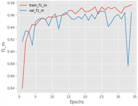
Figure 10. Training and validation F1-score of the proposed mode
The F1 score of the model during training and validation is visualized in Figure 10. The F1 score for the training consistently surpassed the F1 score for validation. In the first five epochs, there was a significant increase in the training F1-score, while the validation F1-score only showed a slight increase. After that, the training and validation values gradually increased until they reached 30 epochs. After 30 epochs, the training F1-score reached its maximum value of 0.98, while the validation F1-score fluctuated before eventually reaching a value of 0.96.
4.3 Testing results
There are various types of pneumonia, including aspiration, bacterial, and viral pneumonia, which can all manifest differently on radiography. An incorrect diagnosis could result from a model that is poorly trained to recognize one kind (e.g., bacterial) not generalizing to other types (e.g., viral). Specifically, models trained on datasets including more common neumonia cases may not identify the distinct characteristics that COVID-19 pneumonia exhibits. Furthermore, certain models may overfit the training set, which results in good performance on the training dataset but poor performance on new, untested data. The inability of the model to generalize to more individuals is made worse by small or homogeneous datasets. In this paper, after training and validating the model, it was tested on new images from the testing dataset to assess its performance on previously unseen images.
Table 3. Performance evaluation on testing dataset
|
|
Accuracy |
F1 Score |
Recall |
Precision |
|
Test set |
0.9578 |
0.9719 |
0.9844 |
0.9596 |
According to Table 3, the model demonstrated a high level of accuracy, achieving a value of 0.957 on the testing dataset. Furthermore, the values of the recall (0.98), precision (0.95), and F1 score (0.97) were all high. The results demonstrated that the model has a high accuracy in identifying the presence of pneumonia in chest X-rays, as well as classifying normal chest X-rays.
Figure 11. Random selection of predictions in testing dataset
Figure 12. ROC curve for testing
Figure 11 is an example of the predictions that were performed by the model to classify chest X-ray images into pneumonia or normal.
Furthermore, the model was evaluated according to AUC (shown in Figure 12), where the AUC value was 0.99. This high AUC score demonstrates the models’ capability in discriminating between negative and positive cases with high FP and TP rates.
4.4 Comparison with other models
The use of the proposed RN50 CNN-AFDA model gave promising results with a high value of ROC curve of 0.99; this ascertains its high accuracy in discriminating between the two classes, namely the positive and negative ones. In addition, the proposed method had better performance in the classification of pneumonia with accuracy of 0.957 and average F1-score of 0.97. The results for the proposed TL-ResNet50-CNN model are favorable compared to the study conducted by Singh et al. [26] since the proposed model showed better accuracy (0.957) compared to the accuracy of 0.9375 identified in the study by Singh et al. [26]. In addition, the ROC curve results were 0.99 for the proposed model compared to 0.96 obtained by Singh et al. [26]. Therefore, the proposed TL-ResNet50 model was compared to other recently published models in terms of performance and observed to outperform the other related methods by achieving a higher accuracy and F1-score as depicted in Table 4.
Table 4. Comparison of the performance of the proposed model with existing DL models
|
S/No. |
Architecture |
Accuracy |
F-Score |
Recall |
Precision |
|
- |
Proposed Model |
0.957 |
0.97 |
0.9844 |
0.9596 |
|
[3] |
Fuzzy Expected Value |
44.6 |
92.7 |
84.1 |
96.7 |
|
[26] |
VGG16 |
92.14 |
0.9234 |
-- |
-- |
|
VGG19 |
90.22 |
0.8999 |
-- |
-- |
|
|
ResNet50 |
82.37 |
0.8281 |
-- |
-- |
|
|
ResNet101 |
75.96 |
0.7593 |
-- |
-- |
|
|
ResNet152 |
87.179 |
0.8734 |
-- |
-- |
|
|
ResNet50V2 |
89.26 |
0.8937 |
-- |
-- |
|
|
ResNet101V2 |
92.62 |
0.925 |
-- |
-- |
|
|
ResNet152V2 |
92.94 |
0.9312 |
-- |
-- |
|
|
InceptionV3 |
89.42 |
0.8937 |
-- |
-- |
|
|
InceptionResNetV2 |
90.7 |
0.8989 |
-- |
-- |
|
|
DenseNet121 |
91.82 |
0.9171 |
-- |
-- |
|
|
DenseNet169 |
88.78 |
0.8874 |
-- |
-- |
|
|
DenseNet201 |
91.83 |
0.9171 |
-- |
-- |
|
|
NASNetLarge |
88.14 |
0.8812 |
-- |
-- |
|
|
Quaternion Residual Network |
93.75 |
0.9405 |
-- |
-- |
A novel RN50 CNN-AFDA scheme for the classification of chest X-ray images into Pneumonia and Normal classes was designed and implemented in this study based on the Adaptive Fractional Differential Algorithm; the evaluation was done using pneumonia X-ray dataset sourced from the Mendeley data repository. The dataset was first pre-processed before the training and testing phases. From the evaluations, the proposed scheme made the following contributions:
High accuracy: The proposed model achieved high accuracy of 95% following the evaluations with an F1 score of 0.97, proving the effectiveness of the proposed ResNet50 in the detection of pneumonia.
Applicability on large datasets: Another disadvantage of other models which are oriented on pneumonia detection is that those models are trained and tested with small sets of data. On the other hand, the proposed RN50 CNN-AFDA scheme used in this paper was trained and tested on a larger image database of 5856 images. This way, the model acquires better generalization capacity and the possibility to be less susceptible to over-fitting.
Superiority to other models: The proposed RN50 CNN-AFDA scheme performs higher accuracy of the test cases with a better F1 score than other related works that focused on the application of ML and DL methods to pneumonia detection.
Time efficiency: The proposed RN50 CNN-AFDA scheme provides a fast method of producing much faster outcomes based on the chest X-rays; this is in contrast to slow and time-consuming method of analysis by specialized physicians handling the films. Hence, the proposed method could hasten early identification and possibly early intervention of cases of pneumonia.
Generalized applicability in the health sector: The presented RN50 CNN-AFDA showed excellent performance in the detection process of the images of the X-rays. In general, the procedure of obtaining such a model does not depend on the specific purpose of using it in the medical field; hence, the proposed model can also be applied in other medical fields for spotting other diseases based on images.
The suggested scheme demonstrates promise for generalization when tested on various data sets. The future scope of the proposed study is predicted to yield better outcomes if the suggested architecture is combined with the expert radiologists' projections.
[1] Li, B., Xie, W. (2015). Adaptive fractional differential approach and its application to medical image enhancement. Computers & Electrical Engineering, 45: 324-335. https://doi.org/10.1016/j.compeleceng.2015.02.013
[2] Zerunian, M., Pucciarelli, F., Caruso, D., Polici, M., et al. (2022). Artificial intelligence based image quality enhancement in liver MRI: A quantitative and qualitative evaluation. La Radiologia Medica, 127(10): 1098-1105. https://doi.org/10.1007/s11547-022-01539-9
[3] Alzahrani, A., Bhuiyan, M.A.A., Akhter, F. (2022). Detecting COVID-19 pneumonia over fuzzy image enhancement on computed tomography images. Computational and Mathematical Methods in Medicine, 2022(1): 1043299. https://doi.org/10.1155/2022/1043299
[4] Ortiz-Toro, C., Garcia-Pedrero, A., Lillo-Saavedra, M., Gonzalo-Martin, C. (2022). Automatic detection of pneumonia in chest X-ray images using textural features. Computers in Biology and Medicine, 145: 105466. https://doi.org/10.1016/j.compbiomed.2022.105466
[5] Ukwuoma, C.C., Qin, Z., Heyat, M.B.B., Akhtar, F., et al. (2023). A hybrid explainable ensemble transformer encoder for pneumonia identification from chest X-ray images. Journal of Advanced Research, 48: 191-211. https://doi.org/10.1016/j.jare.2022.08.021
[6] Ibrahim, R.W., Jalab, H.A., Karim, F.K., Alabdulkreem, E., Ayub, M.N. (2022). A medical image enhancement based on generalized class of fractional partial differential equations. Quantitative Imaging in Medicine and Surgery, 12(1): 172. https://doi.org/10.21037/qims-21-15
[7] Oldham, K., Spanier, J. (1974). The Fractional Calculus Theory and Applications of Differentiation and Integration to Arbitrary Order. Elsevier.
[8] Nakib, A., Schulze, Y., Petit, E. (2012). Image thresholding framework based on two-dimensional digital fractional integration and Legendre moments’. IET Image Processing, 6(6): 717-727. https://doi.org/10.1049/iet-ipr.2010.0471
[9] Li, B., Xie, W. (2014). Adaptive fractional differential algorithm based on Otsu standard. In the 26th Chinese Control and Decision Conference (2014 CCDC), Changsha, China, pp. 2020-2025. https://doi.org/10.1109/CCDC.2014.6852500
[10] Zhang, X., Liu, R., Ren, J., Gui, Q. (2022). Adaptive fractional image enhancement algorithm based on rough set and particle swarm optimization. Fractal and Fractional, 6(2): 100. https://doi.org/10.3390/fractalfract6020100
[11] Zhang, J., Wei, Z., Xiao, L. (2014). A fast adaptive reweighted residual-feedback iterative algorithm for fractional-order total variation regularized multiplicative noise removal of partly-textured images. Signal Processing, 98: 381-395. https://doi.org/10.1016/j.sigpro.2013.12.009
[12] Zhang, Y., Liu, T., Yang, F., Yang, Q. (2022). A study of adaptive fractional-order total variational medical image denoising. Fractal and Fractional, 6(9): 508. https://doi.org/10.3390/fractalfract6090508
[13] Pu, Y.F., Zhou, J.L., Yuan, X. (2009). Fractional differential mask: A fractional differential-based approach for multiscale texture enhancement. IEEE Transactions on Image Processing, 19(2): 491-511.
[14] Ambroggio, L., Cotter, J., Hall, M., Shapiro, D.J., et al. (2023). Management of pediatric pneumonia: A decade after the pediatric infectious diseases society and infectious diseases society of America guideline. Clinical Infectious Diseases, 77(11): 1604-1611. https://doi.org/10.1093/cid/ciad385
[15] Szepesi, P., Szilágyi, L. (2022). Detection of pneumonia using convolutional neural networks and deep learning. Biocybernetics and Biomedical Engineering, 42(3): 1012-1022. https://doi.org/10.1016/j.bbe.2022.08.001
[16] Yoon, T., Kang, D. (2024). Enhancing pediatric pneumonia diagnosis through masked autoencoders. Scientific Reports, 14(1): 6150. https://doi.org/10.1038/s41598-024-56819-3
[17] Zhang, Y., Yang, L., Li, Y. (2022). A novel adaptive fractional differential active contour image segmentation method. Fractal and Fractional, 6(10): 579. https://doi.org/10.3390/fractalfract6100579
[18] Diethelm, K., Ford, N.J. (2004). The Analysis of Fractional Differential Equations. Springer.
[19] Teodoro, G.S., Machado, J.T., De Oliveira, E.C. (2019). A review of definitions of fractional derivatives and other operators. Journal of Computational Physics, 388: 195-208. https://doi.org/10.1016/j.jcp.2019.03.008
[20] Swab, M. (2016). Mendeley data.Journal of the Canadian Health Libraries Association/Journal de l'Association des Bibliothèques de la Santé du Canada, 37(3): 121-123.
[21] He, K., Zhang, X., Ren, S., Sun, J. (2016). Deep residual learning for image recognition. In 2016 IEEE Conference on Computer Vision and Pattern Recognition (CVPR), Las Vegas, USA, pp. 770-778. https://doi.org/10.1109/CVPR.2016.90
[22] Kingma, D.P. (2014). Adam: A method for stochastic optimization. arXiv preprint arXiv:1412.6980. https://doi.org/10.48550/arXiv.1412.6980
[23] Lu, J., Steinerberger, S. (2022). Neural collapse under cross-entropy loss. Applied and Computational Harmonic Analysis, 59: 224-241. https://doi.org/10.1016/j.acha.2021.12.011
[24] Naser, Z.S., Khalid, H.N., Ahmed, A.S., Taha, M.S., Hashim, M.M. (2023). Artificial neural network-based fingerprint classification and recognition. Revue d'Intelligence Artificielle, 37(1): 129-137. https://doi.org/10.18280/ria.370116
[25] Schnawa, S.A., Rafie, M., Taha, M.S. (2023). DAE-DBN: An effective lung cancer detection model based on hybrid deep learning approaches. In International Conference of Reliable Information and Communication Technology, Johor Bahru, Malaysia, pp. 108-118. https://doi.org/10.1007/978-3-031-59711-4_10
[26] Singh, S., Kumar, M., Kumar, A., Verma, B.K., Shitharth, S. (2023). Pneumonia detection with QCSA network on chest X-ray. Scientific Reports, 13(1): 9025. https://doi.org/10.1038/s41598-023-35922-x