Siska Yosmar* | Septri Damayanti | Jose Rizal
© 2025 The authors. This article is published by IIETA and is licensed under the CC BY 4.0 license (http://creativecommons.org/licenses/by/4.0/).
OPEN ACCESS
The Sumatra subduction zone is a highly active tectonic region with significant stress accumulation, making it prone to potentially devastating earthquakes. Accurate forecasting of earthquake frequency in this area is crucial for disaster preparedness and risk mitigation. This study applies Singular Spectrum Analysis (SSA), a non-parametric method, to model and predict earthquake occurrences. To evaluate the reliability of SSA, four data division cases were tested: Case 1, with 80% training data and 20% testing data; Case 2, with 85% training data and 15% testing data; Case 3, with 90% training data and 10% testing data; and Case 4, with 95% training data and 5% testing data. Among these, Case 3 provided the most accurate representation of historical data, achieving the lowest Root Mean Square Error (RMSE) and Mean Arctangent Absolute Percentage Error (MAAPE) values for in-sample predictions. However, no definitive conclusion could be drawn regarding the best composition for out-sample predictions. These insights highlight the importance of testing models across different data splits to ensure reliable forecasting. This approach offers a valuable tool for planning and preparedness in earthquake-prone regions.
earthquake forecasting, subduction zone, Singular Spectrum Analysis, time series modeling, accuracy metrics
Earthquakes are among the most destructive natural disasters, particularly in Indonesia, which lies at the intersection of the Eurasian, Indo-Australian, and Pacific tectonic plates. The Sumatra subduction zone is one of the most seismically active regions globally, characterized by frequent tectonic activity and significant stress accumulation. Accurate prediction of earthquake frequency in this region is essential for disaster preparedness and risk mitigation. However, traditional time series modeling techniques, such as Autoregressive Integrated Moving Average (ARIMA) and Generalized AutoRegressive Conditional Heteroskedasticity (GARCH), often face limitations due to their reliance on assumptions of linearity and stationarity. These methods struggle to capture the dynamic and irregular characteristics of earthquake occurrences. Machine learning approaches, while offering some promise, often require extensive datasets and lack transparency, making it challenging to interpret underlying patterns in earthquake frequency. Although technology has advanced, it still cannot predict the exact time and location of an earthquake. However, areas prone to earthquakes and their potential impacts have been mapped. The annual earthquake frequency data can be used as a basis for prediction through time series analysis. Various methods have been applied in earthquake time series analyses to estimate the frequency of earthquakes using this data.
This study introduces SSA as a novel and effective approach to earthquake frequency modeling, particularly for the complex dynamics of the Sumatra subduction zone. SSA’s ability to decompose and reconstruct non-linear and non-stationary time series data provides a significant advantage over traditional methods. By breaking down complex seismic data into trend, periodic, and noise components, SSA can reveal underlying patterns that are often obscured in traditional analyses. Furthermore, this study evaluates SSA’s robustness through various insample-outsample data splits, demonstrating its capability to adapt to different data configurations and ensure reliable forecasting. By applying SSA to earthquake frequency modeling, this research not only fills a critical methodological gap but also contributes valuable insights into seismic hazard assessment and disaster risk reduction strategies in one of the world’s most vulnerable regions.
This study makes several key contributions to earthquake frequency modeling and disaster preparedness. First, it demonstrates the effectiveness of SSA as a forecasting tool for earthquake frequency. By applying SSA to complex, non-linear, and non-stationary seismic data, the study reveals its ability to decompose and reconstruct meaningful patterns, offering a robust alternative to traditional methods that often struggle with such challenging data characteristics. Subsequently, the research evaluates SSA’s performance across various in-sample and out-of-sample data splits, providing valuable insights into the best data configurations for accurate forecasting. This analysis confirms the robustness and adaptability of SSA in different data scenarios, enhancing its practical applicability. Finally, the study contributes to disaster preparedness by providing actionable insights for seismic hazard assessment in the Sumatra subduction zone one of the most seismically active regions in the world. The findings have the potential to inform early warning systems and improve resource allocation strategies, ultimately strengthening mitigation efforts in earthquake-prone areas.
In this study, the data is divided into in-sample and out-of-sample sets with varying proportions to evaluate the reliability of the SSA method. The data is split into four different cases: Case 1 with 80% training data and 20% testing data, Case 2 with 85% training data and 15% testing data, Case 3 with 90% training data and 10% testing data, and Case 4 with 95% training data and 5% testing data. This approach ensures that the analysis method is thoroughly tested across different data configurations, helping to produce models that provide accurate and reliable predictions. It is important to note that earthquakes with a magnitude below the Magnitude of Completeness (Mc) were excluded from the analysis.
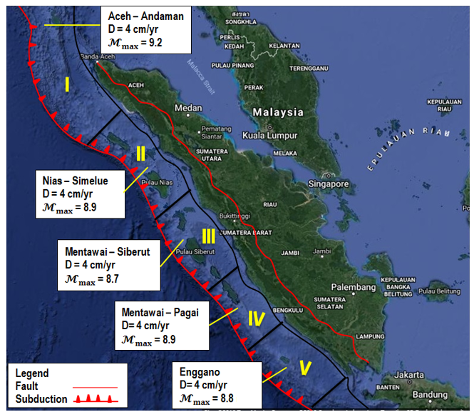
The island of Sumatra is located along the collision path of two tectonic plates, namely the India-Australia Plate and the Eurasian Plate. The boundary of the collision of these two plates is clearly visible in the form of a deep-sea trench in the west of Sumatra to the Andaman Islands, where the India-Australia Plate infiltrates under the island of Sumatra at a speed of 50-60 mm/year and a slope of about 12 degrees to the east [1]. The National Center for Earthquake Studies (PuSGeN) as one of the forums for researchers on seismicity in Indonesia has succeeded in identifying several 4 segments of large earthquake sources in the Sumatra megathrust zone, namely the Aceh-Andaman (AA), Nias-Simeuleu (NS), Mentawai-Pagai (MP), Mentawai-Siberut (MS), and Enggano (EO) segments. Visually, the limitations of the five segments of the source of the large earthquake can be seen in Figure 1 [2]. In the figure, information about the identity of the segment, the maximum potential earthquake is displayed, and the shear rate of tectonic plates in cm/year.
Figure 1. Source segment in the Sumatra megathrust zone
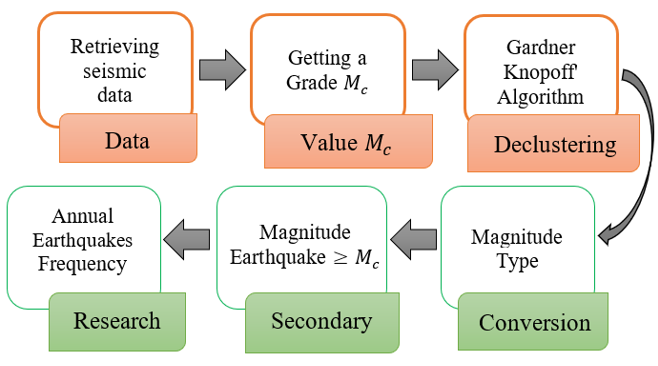
Figure 2. Research data preparation process
The data used in this study is mainshock earthquake. To obtain this data, a data preparation stage is required. The data preparation stage in this study uses the help of the ZMapp 7.1 package on MATLAB R2018a software and Microsoft Excel which follows the procedure as shown in Figure 2.
The first stage of research data preparation is to obtain data on earthquake events from January 1st, 1900 to December 31st, 2023. The data collection was carried out using the help of the ZMapp 7.1 package on the MATLAB R2018a software. In the process of collecting earthquake data using the ZMapp 7.1 package using a source from the USGS for the subduction zone of Sumatra Island with latitude (6° LU-11° LS) and longitude (94° BT-105° BT). The data to be taken is magnitude 2.5 until 10 Mw with a depth of ≤70 km. One of the reasons for choosing the depth of the earthquake is because an earthquake with this depth has the potential to cause great damage and can trigger a tsunami wave after an earthquake.
After knowing the value of M_c then the declustering process will be carried out. Declustering is the process of separating earthquake events between the main earthquake (mainshock) and the pioneer earthquake (foreshock), and aftershocks [3]. In this study, the declustering process uses the GardnerKnopoff method. GardnerKnopoff declustering is a method to separate pioneer or minor earthquakes that occur in groups or within the same time and location from major or large earthquakes in a short span of time [4]. The main goal of GardnerKnopoff declustering is to identify and remove shear earthquakes that occur due to major earthquake activity, thereby improving accuracy in statistical analysis and earthquake modeling. The GardnerKnopoff method is based on two assumptions, namely the assumption that major earthquakes can trigger pilot or minor earthquakes in a short span of time with the same location and the assumption that the time and location of pilot earthquakes can be considered as random variables [5]. The subsequent process is the uniformity of the magnitude type into one scale in the magnitude type M_w and sorting data with the provision data of value ≥M_c.
2.1 SSA
SSA is one of the time series data analysis techniques used for forecasting. As we know, the SSA method is a non-parametric technique used to observe a time series data that is not linear, not stationary, has a variable nature at any time or temporarily, and more prone to success for short time-series [6, 7]. In general, SSA combines elements of classical time series analysis, multivariate statistics, multivariate geometry, dynamical systems, and signal processing. SSA can be very useful in solving various problems such as forecasting, imputation of missing values, decomposition of the original time series into a small number of interpretable components such as slowly changing trends, oscillatory components, and unstructured noise [8]. In SSA, the segmentation procedure produces smaller time series, which is favorable for SSA. If a time-series is non-stationary, transient oscillations can be evidenced locally in a given segment, whereas they could go unnoticed in the general computation of the whole time-series [9].
The main steps in forecasting using the SSA method are: Decomposition: The time series data is converted into a matrix (trajectories) using a window length parameter. This matrix is split using Singular Value Decomposition (SVD) into principal components that represent different patterns. Reconstruction: Relevant components are selected based on their contribution or significance (usually those with the largest singular values). These components are then recombined to reconstruct the time series into trends, seasonality, or noise as per the analysis. Forecasting: Based on the reconstructed components, a model is built to extend (forecast) the time series into the future while maintaining the identified patterns [6, 9]. The purpose of the first stage, decomposition, is to decompose the original series into a small number of independent and interpretable components such as slowly varying trends, oscillatory components, and unstructured noise. At this stage, capabilities for vibration analysis will also be applied. Then, in the second stage, reconstruction will be used to reconstruct the original signal using a selected number of components. For example, one can select only a certain number of components that contain important signal features, such as trend and oscillation components, and discard the (unstructured) noise components that cause discrepancies in the analysis results [10].
2.1.1 Embedding
Embedding is a stage where the initial time series data is converted into a trajectory X matrix, meaning converting the initial data in the form of one-dimensional data into multidimensional data. The trajectory X matrix has dimensions L×K. L shows the window length in the X matrix which is the number of rows, while K indicates the number of columns in the matrix. The selection of an appropriate value of the window length L is of great importance in SSA operation. This is because the efficiency of SSA in separating different signal components from the composite signal depends on the value of L [11].
In practice, the selection of window length (L) and clustering strategy are critical for optimal analysis results. The window length is usually chosen between 2 to N/2 (where N is the length of the data) and is tailored to the nature of the data: if the data has periodic patterns, the L should be close to a multiple of the period to capture seasonal patterns, while for data with dominant trends, a larger L is more suitable. The clustering strategy is performed after decomposition, where component clustering will be performed based on patterns, such as smooth components with large singular values for trends, oscillating components for seasonality, and components with random fluctuations and small singular values for noise.
There is no special method to determine the value of L precisely, so to determine the value of L is done by trial and error for the value to be in the range 2≤L≤2-1 N and the time series data throughout the period N does not contain missing data and X={xi}; i=1,2,…,N. Furthermore, in determining the value of K by K=N-L+1, where, N is the amount of data and L is the length of the windows [12]. The X trajectory matrix formed is a Hankel matrix where all its anti-diagonal elements have constant values. In the form of a matrix, it can be expressed as follows:
$\boldsymbol{X}=\left[x_1, x_2, \ldots, x_N\right]=\left[\begin{array}{ccccc}x_1 & x_2 & x_3 & \ldots & x_K \\ x_2 & x_3 & x_4 & \ldots & x_{K+1} \\ x_3 & x_4 & x_5 & \ldots & x_{K+2} \\ \vdots & \vdots & \vdots & \ddots & \vdots \\ x_L & x_{L+1} & x_{L+2} & \ldots & x_{L K}\end{array}\right]$ (1)
2.1.2 Singular Value Decomposition (SVD)
The SVD stage in its application has similarities with principal component analysis, which is to reduce components from the initial data and reduce dimensions [13]. The purpose of SVD is to obtain the separation of components in decomposition from time series data. Due to the high computational cost associated with SVD, its application to large datasets may not be suitable [14]. Note that, SVD begins with determining eigenvalue values $\left(\lambda_1, \lambda_2, \lambda_3, \ldots \lambda_L\right)$ from the matrix $\mathbf{S}=\mathbf{X} \mathbf{X}^{\mathrm{T}}$ where $\lambda_1 \geq \lambda_2 \geq \lambda_3 \geq \cdots \geq \lambda_L>0$, and eigenvector $\left(u_1, u_2, u_3, \ldots, u_L\right)$ from the $S$ matrix. The eigenvalue and eigenvector calculations of the $S$ matrix can be done using the following definitions:
Definition 1. If A is a matrix n×n, then the non-zero vector x is inside, Rn. called an eigenvector (vector eigen) of A if Ax is a scalar multiple of x; that is
$\boldsymbol{A} x=\lambda x$
for a scalar λ. The scalar λ is called the eigenvalue of A and x is said to be the eigenvalue corresponding to λ [15].
To determine the eigenvalue of the $\boldsymbol{S}$ matrix measuring $L \times L$, so $\boldsymbol{A} x=\lambda x$ as $\boldsymbol{S} x=\lambda I x$ where in this case the matrix $\boldsymbol{S}$ is the matrix $\boldsymbol{A}$ referred to in Definition 1. The equation is equivalent to $(\lambda I-\boldsymbol{S}) x=0$. Thus, for the eigenvalue $\lambda$ equation $(\lambda I-\boldsymbol{S}) x=0$ has a non-zero if and only if:
$\operatorname{det}(\lambda I-\boldsymbol{S})=0$ (2)
Next, the eigenvalue $\lambda_i$ will be obtained by $i=1,2,3, \ldots, L$ and $U_i=\left(u_1, u_2, u_3, \ldots, u_L\right)$ is the corresponding eigenvector of eigenvalue.
Definition 2. Given $\boldsymbol{X}$ matrix $m \times n$ with rank $r$. The positive eigenvalue of $\sqrt{\boldsymbol{X} \boldsymbol{X}^{\boldsymbol{T}}}$ is called the singular value of $\boldsymbol{X}$ [16].
In other words, if $\sigma$ is the singular value of $X$ then $\sigma$ is the positive eigenvalue of $\sqrt{X X^T}$ or $\sigma^2$ is the eigenvalue of $X X^T$. From Definition 2, the relationship between the eigenvalue and the singular value is obtained. In other words, a singular value matrix is a matrix that is $\mathrm{L} \times \mathrm{K}$ in size with the main diagonal containing the positive root of the eigenvalue $\left(\sqrt{\lambda_i}\right)$ with the order $\lambda_1 \geq \lambda_2 \geq \lambda_3 \geq \ldots \geq \lambda_L>0$. It can be seen from the matrix below:
$\sqrt{\lambda_i}=\left[\begin{array}{ccc}\sqrt{\lambda_1} & \cdots & 0 \\ \vdots & \ddots & \vdots \\ 0 & \cdots & \sqrt{\lambda_L}\end{array}\right]=\left[\begin{array}{ccc}\sigma_1 & \cdots & 0 \\ \vdots & \ddots & \vdots \\ 0 & \cdots & \sigma_L\end{array}\right]=\sigma_i$ (3)
Furthermore, in determining the principal component matrix, can be searched using the relationship of singular values with the left singular vector and the right singular vector as follows:
Definition 3. Suppose the real matrix $\boldsymbol{X}$ is $m \times n$. Positive real numbers $\sigma$ called singular values of matrix $\boldsymbol{X}$ if there are zero vectors $\boldsymbol{U} \in \boldsymbol{R}^{\boldsymbol{m}}$ and $\boldsymbol{V} \in \boldsymbol{R}^{\boldsymbol{n}}$ so that $\boldsymbol{X} \boldsymbol{V}=\sigma \boldsymbol{U}$ and $\boldsymbol{X}^{\boldsymbol{T}} \boldsymbol{U}=\sigma \boldsymbol{V}$. The $U$ vector is called the left singular vector and $\boldsymbol{V}$ is called the right singular vector. Furthermore $(\sigma, U)$ is called the left singular pair of $\boldsymbol{X}$, and $(\sigma, V)$ is called the right singular pair of $\boldsymbol{X}$ [16].
From the above definition, the following equation is obtained:
$\boldsymbol{X} \boldsymbol{V}=\sigma_i \boldsymbol{U}$ and $\boldsymbol{X}^T \boldsymbol{U}=\sigma_i \boldsymbol{V}$
for vectors $\boldsymbol{V}_{\boldsymbol{i}}$ with $i=1,2,3, \ldots, L$ follows the following equation:
$\boldsymbol{V}_i=\frac{\boldsymbol{X}^T \boldsymbol{U}_i}{\sqrt{\lambda_i}}$ (4)
$\boldsymbol{V}_i^T$ is a transpose of the $\boldsymbol{V}_i$ matrix, so that the $\boldsymbol{V}_i^T$ matrix can be written in the form of:
$\boldsymbol{V}_i^T=\left[\begin{array}{cccc}v_{11} & v_{12} & \ldots & v_{1 L} \\ v_{21} & v_{22} & \ldots & v_{2 L} \\ \vdots & \vdots & \ddots & \vdots \\ v_{K 1} & v_{K 2} & \ldots & v_{K L}\end{array}\right]$ (5)
After obtaining the singular value $\left(\sigma_i\right)$, eigenvector $(\boldsymbol{U})$, and principal component $(\boldsymbol{V})$, the decomposition of the singular value of the trajectory matrix $\boldsymbol{X}$ is as follows:
Definition 4. For each $\boldsymbol{X} \in \boldsymbol{\Omega}^{m \times n}$ of rank $r$, there is an orthogonal matrix $\boldsymbol{U}_{m \times m}, V_{n \times n}$ and a diagonal matrix $\boldsymbol{D}_{r \times r}=$ $\operatorname{diag}\left(\sigma_1, \sigma_2, \ldots, \sigma_r\right)$ so that
$\boldsymbol{X}=\boldsymbol{U}\left(\begin{array}{ll}\boldsymbol{D} & \mathbf{0} \\ \mathbf{0} & \mathbf{0}\end{array}\right)_{m \times n} \boldsymbol{V}^T$ (6)
with $\sigma_1 \geq \sigma_2 \geq \cdots \geq \sigma_r>0$ [17].
The $\boldsymbol{V}^{\boldsymbol{T}}$ matrix is a transpose of the $\boldsymbol{V}$ and $\boldsymbol{U}$ matrices of $L \times L$ and $\boldsymbol{D}_{r \times r}$ is a matrix with $L \times K$ dimensions whose main diagonal element is the singular value of the $S$ matrix, so that the value of $X_i$ can be found by the following steps:
$\begin{gathered}\boldsymbol{X}_{\boldsymbol{i}}=\left[\begin{array}{cccc}u_{11} & u_{12} & \ldots & u_{1 L} \\ u_{21} & u_{22} & \ldots & u_{2 L} \\ \vdots & \vdots & \ddots & \vdots \\ u_{L 1} & u_{L 2} & \ldots & u_{L L}\end{array}\right]\left[\begin{array}{cccc}\sigma_1 & 0 & 0 & 0 \\ 0 & \sigma_2 & 0 & 0 \\ 0 & 0 & \ddots & 0 \\ 0 & 0 & 0 & \sigma_L\end{array}\right]\left[\begin{array}{cccc}v_{11} & v_{12} & \ldots & v_{1 k} \\ v_{21} & v_{22} & \ldots & v_{2 K} \\ \vdots & \vdots & \ddots & \vdots \\ v_{K 1} & v_{K 2} & \ldots & v_{K K}\end{array}\right]\\=\boldsymbol{U}_1 \sigma_1 \boldsymbol{V}_1^T+\boldsymbol{U}_2 \sigma_2 \boldsymbol{V}_2^T+\cdots+ \boldsymbol{U}_d \sigma_d \boldsymbol{V}_d^T=\sum_{i=1}^d \boldsymbol{U}_i \sigma_i \boldsymbol{V}_i^T\end{gathered}$ (7)
with $i=1,2,3, \ldots, d$ and $d=\max \{i\}$ and $\sigma_i>0$.
The three components in the $\boldsymbol{X}_{\boldsymbol{i}}$ matrix namely singular value $\left(\sigma_i\right)$, eigenvector $\left(\boldsymbol{U}_i\right)$, and principal component $\left(\boldsymbol{V}_i\right)$ are called the i'th eigentriple of Singular Value Decomposition. So the SVD for the $\boldsymbol{X}_{\boldsymbol{i}}$ matrix can be written as follows [6]:
$\boldsymbol{X}_i=\boldsymbol{X}_1+\boldsymbol{X}_2+\boldsymbol{X}_3+\cdots+\boldsymbol{X}_d$. (8)
2.2 Reconstruction
Reconstruction is a stage where the data is reconstructed into new time series data based on the values obtained in the previous stage, namely the decomposition stage [6]. The newly obtained time series data will go through two processes, namely grouping and diagonal averaging.
2.2.1 Grouping
Grouping is the grouping of a matrix of $\boldsymbol{X}_i$ into several groups. The grouping of the $\boldsymbol{X}_{\boldsymbol{i}}$ matrix can be done by subjectively looking at eigentriple value patterns or can perform spectral analysis to see patterns and periods in eigentriples. The grouping process is carried out by grouping the set of indices $\{1,2,3, \ldots, d\}$ into $m$ subsets denoted by $I=$ $I_1, I_2, I_3, \ldots, I_m$ with $d=m$. Then $\boldsymbol{X}_I$ adjusted to the group $I=\left\{I_1, I_2, I_3, \ldots, I_m\right\}$. Then $\boldsymbol{X}_i=X_1, X_2, X_3, \ldots, \boldsymbol{X}_m$ can be expanded to:
$\boldsymbol{X}_I=\boldsymbol{X}_{I 1}+\boldsymbol{X}_{I 2}+\boldsymbol{X}_{I 3}+\cdots+\boldsymbol{X}_{I m}$. (9)
The stage to select the set $\mathrm{I}=\left\{\mathrm{I}_1, \mathrm{I}_2, \mathrm{I}_3, \ldots, \mathrm{I}_{\mathrm{m}}\right\}$ is called eigentriple grouping which is carried out by trial and error. The trial-and-error method can be done subjectively, that is, trying all possibilities by looking at the correlation plot or relationship of each eigentriple.
The concept of forecasting in the SSA method is a separation that characterizes how well different components can separate from each other. The decomposition of SSA from FN series will only be successful if the additive components of the series can be separated from each other. The natural measurement of similarity between two series X(1) and X(2) uses the W–correlation equation which is formulated as follows [6]:
$\rho^{(w)}\left(\mathbb{X}^{(1)}, \mathbb{X}^{(2)}\right)=\frac{\left(\mathbb{X}^{(1)}, \mathbb{X}^{(2)}\right)_w}{\left\|\mathbb{X}^{(1)}\right\|_w\left\|\mathbb{X}^{(2)}\right\|_w}$ (10)
with $\left(\mathbb{X}^{(1)}, \mathbb{X}^{(2)}\right)_w=\sum_{i=0}^N w_i x_i^{(1)} x_i^{(2)}$ and $w_i$ searched by using:
$w_i=\left\{\begin{array}{c}i \quad \text { for } 0 \leq i<L^* \\ L^* \quad \text { for } L^* \leq i \leq K^* \\ N-i+1 \text { for } K^*<i \leq N\end{array}\right.$
with $L^*=\min (L, K)$ and $K^*=\max (L, K)$.
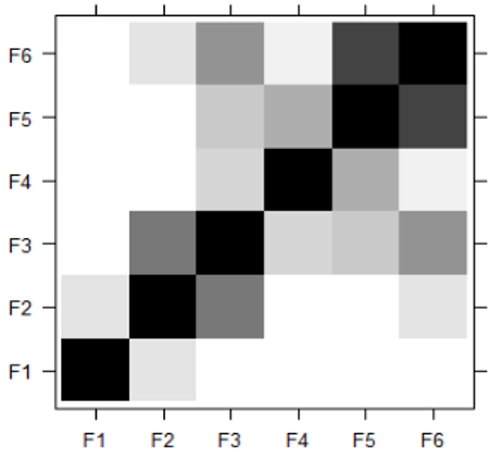
Figure 3. Example of W-correlation plot
If the absolute value of W-correlation is small, then the series almost meets the W-orthogonal. On the contrary, the sequence is far from the W-orthogonal and is very separate. So, if both reconstructed components have a W-correlation value of zero, it means that the two components can be separated. The W-correlation plot is used as a visualization of the magnitude of the correlation between eigentriples [6]. The older the color, the higher the correlation. An example of a W-correlation plot can be seen in Figure 3.
2.2.2 Diagonal averaging
After grouping, the next stage will be transformed from the grouping results, namely diagonal averaging. This step is done by converting each matrix $\boldsymbol{X}_I$ into a new time series with a length of $N$. Suppose the matrix $\boldsymbol{F}$ is an arbitrary matrix of $\mathrm{L} \times \mathrm{K}$ size with $f_{i j}$ elements with $1 \leq \mathrm{i} \leq \mathrm{L}$ and $1 \leq \mathrm{j} \leq \mathrm{K}, L^*=$ $\min (L, K), K^*=\max (L, K)$, and $N=L+K-1$.
$\boldsymbol{F}=\left[\begin{array}{ccccc}f_{11} & f_{12} & f_{13} & \ldots & f_K \\ f_{21} & f_{22} & f_{23} & \ldots & f_{K+1} \\ f_{31} & f_{32} & f_{33} & \ldots & f_{K+2} \\ \vdots & \vdots & \vdots & \ddots & f_{K+3} \\ f_L & f_{L+1} & f_{L+2} & \ldots & f_N\end{array}\right]$ (11)
The matrix $\boldsymbol{F}$ is transformed into a series of $g_1, g_2, g_3, \ldots, g_N$ through diagonal averaging with the following formula [6]:
$g_k=\left\{\begin{array}{l}\frac{1}{k+1} \sum_{m=1}^{k+1} y_{m, k-m+1}^*, \text { for } 0 \leq k<L^*-1 \\ \frac{1}{L^*} \sum_{m=1}^{L^*} y_{m, k-m+2}^*, \text { for } L^*-1 \leq k<K^* \\ \frac{1}{N-k} \sum_{m=k-K^*+2}^{N-K^*+1} y_{m, k-m+2}^*, \text { for } K^* \leq k<N\end{array}\right.$ (12)
Based on Eqs. (11) and (12), for example, in the matrix $\boldsymbol{F}$ is chosen for $k=1$ to give the result $g_1=f_{11}$, for $k=2$ gives $g_2=\frac{f_{12}+f_{21}}{2}$, for $k=3$ gives $g_3=\frac{f_{13}+f_{22}+f_{31}}{3}$ and so on. Meanwhile, based on Eq. (12), if applied to the $X_{I m}$ resultant matrix, a series $\tilde{g}^{(k)}=\left(\tilde{g}_1^{(k)}, \tilde{g}_2^{(k)}, \ldots, \tilde{g}_N^{(k)}\right)$ so that the original series is decomposed into:
$g_k=\left\{\begin{array}{l}\frac{1}{k+1} \sum_{m=1}^{k+1} y_{m, k-m+1}^*, \text { for } 0 \leq k<L^*-1 \\ \frac{1}{L^*} \sum_{m=1}^{L^*} y_{m, k-m+2}^*, \text { for } L^*-1 \leq k<K^* \\ \frac{1}{N-k} \sum_{m=k-K^*+2}^{N-K^*+1} y_{m, k-m+2}^*, \text { for } K^* \leq k<N\end{array}\right.$ (13)
2.3 Linear Recurrent Formula (LRF)
Forecasting in the SSA method uses LRF or known as R-Forecasting. SSA-LRF is a non-parametric method that is widely used for time series forecasting and does not accommodate random behavior (noise) in the analysis set because the goal is to separate the signal from the noise component [18]. The time series used is the value of the reconstruction series obtained from the averaging diagonal results. R-Forecasting forecasting is related to the estimation of the LRF, namely $a_1, a_2, a_3, \ldots, a_d$ which is an eigenvector obtained from the SVD stage [19]. The prediction model is as follows:
$g_i=\left\{\begin{array}{c}\tilde{y}_l, \quad i=0,1,2, \ldots, N \\ \sum_{j=1}^{L-1} a_j g_{i-j}, i=N+1, N+2, \ldots, N+M\end{array}\right.$ (14)
If for example $\boldsymbol{U}=\left(\boldsymbol{u}_1, \boldsymbol{u}_2, \boldsymbol{u}_3, \ldots, \boldsymbol{u}_{\boldsymbol{L}-1}, \boldsymbol{u}_L\right)^{\boldsymbol{T}}, \boldsymbol{U}^{\boldsymbol{\nabla}}=$ $\left(\boldsymbol{u}_1, \boldsymbol{u}_2, \boldsymbol{u}_3, \ldots, \boldsymbol{u}_{L-1}\right)^{\boldsymbol{T}}$, and $\boldsymbol{\pi}_{\boldsymbol{i}}$ is the last component of the eigenvector $\boldsymbol{U}$ or can be written $\pi_i=u_L$ then the LRF coefficient can be calculated [19]:
$\mathfrak{R}=U=\left(a_{L-1}, \ldots, a_2, a_1\right)^T=\frac{1}{1-v^2} \sum_{i=1}^r \pi_i \boldsymbol{U}_i^{\nabla}$ (15)
with $v^2=\sum_{i=1}^r \pi_i^2$.
Furthermore, based on Eq. (14), a series of forecasting results will be formed which are shown as follows:
$G_{N+M}=\left(g_1, g_2, g_3, \ldots, g_{N+M}\right)$ (16)
2.4 Forecasting reliability
Point forecast accuracy measures vary based on (i) the type of error (e.g., absolute or squared) considered for their calculation, (ii) the type of scaling (e.g., mean of the series, first differences of the series, or relative performance against a benchmark method) potentially used for making them scale-independent, and (iii) the operator (e.g., mean, median, or geometric mean) utilized for aggregating the errors across different forecast horizons and series [20].
The degree of accuracy of forecasting methods can be explained by comparing the values obtained from forecasting with actual values. The accuracy of a forecasting method is determined by the smallest value of each method, the smaller the error value, the more accurate a method is in forecasting. To measure forecasting accuracy, two popular measures can be used, namely RMSE and MAAPE.
2.4.1 Root Mean Square Error (RMSE)
RMSE is the sum of squared errors or the difference between the actual value and the predicted value that has been determined. The equation for RMSE is as follows [21]:
$R M S E=\sqrt{\sum \frac{\left(g^{\prime}-g\right)^2}{n}}$ (17)
2.4.2 Mean Arctangent Absolute Percentage Error (MAAPE)
MAAPE is a new measure of accuracy developed by observing Mean Absolute Percentage Error (MAPE) from different perspectives. MAAPE measure is the slope as an angle, while MAPE is a slope as a ratio, considering that a triangle with adjacent and opposite sides is equal to the real value and the difference between the actual value and the prediction of each [22].
$M A A P E=\frac{1}{n} \sum_{i=1}^n \arctan \left|\frac{g_i-\hat{g}_i}{g_i}\right|$ (18)
In addition to using these two accuracy measures, in this study, tests will be carried out on residual white noise in the form of residual white noise test and normally distributed residual test which can be seen as follows [23]:
2.4.3 Residual white noise test
The residual white noise test is written as follows:
a. Hypothesis
$\mathrm{H}_0: \rho_1=\rho_2=\cdots=\rho_k=0$ (no residual autocorrelation)
$\mathrm{H}_1$: There is at least one $\rho_{{j}} \neq 0$ (there is a residual autocorrelation)
b. Test statistics, namely Ljung-Box or Box-Pierce Modified test statistics:
$Q^*=n(n+2) \sum_{k=1}^K \frac{\hat{\rho}_k^2}{(n-k)}$ (19)
c. Decision-making criteria:
If the p-value is > alpha (the level of significance set), then H_0 is accepted and it can be concluded that there is no significant residual autocorrelation whereas if the p-value is ≤ alpha, then H_0 rejected and it can be concluded that there is a significant residual autocorrelation. If there is no significant residual autocorrelation, then the model is considered suitable for the data and is good at forecasting.
2.4.4 Normally distributed residual test
In data analysis, given that various statistical methods assume that the distribution of the population data is normal distribution, it is essential to check and test whether or not the data satisfies the normality requirement [24]. The Anderson-Darling test is a modification of the Kolmogorov-Smirnov test. The critical values in the Kolmogorv-Smirnov test do not depend on the specific distribution being tested, whereas the Anderson-Darling test makes use of a specific distribution. In the Anderson-Darling test, the hypothesis used is:
$\mathrm{H}_0$: Residual is normally distributed
$\mathrm{H}_1$: Residual is not normally distributed
The decision is that if the p-value is ≤α, then H_0 rejected and it can be concluded that the residual distribution of the model is not normal while if the p-value>α (the level of significance), then $\mathrm{H}_0$ accepted, that is, the residual distribution of the model is normal [25]. In this case, it can be considered that the model is suitable for the data modeled.
3.1 Forecasting on Case 1
The insample data in Case 1 was converted into 100 one-dimensional data from 1900 to 1999 with the following arrangement:
$\left[\begin{array}{c}\text { Year 1900 } \\ \text { Year 1901 } \\ \text { Year 1902 } \\ \vdots \\ \text { Year 1999 }\end{array}\right]=\left[\begin{array}{c}x_1 \\ x_2 \\ x_3 \\ \vdots \\ x_{100}\end{array}\right]=\left[\begin{array}{c}0 \\ 0 \\ 0 \\ \vdots \\ 58\end{array}\right]$
After the data is converted into one dimension, then converted into multidimensional one called the X trajectory matrix in size L×K. The optimal windows length (L) value is taken based on the smallest forecast accuracy value with an L value range between 2≤L≤50, using the grid method by trying the L values of 5, 10, 15, 20, 25, 30, 35, 40, 45, 45, 50 as shown in Table 1.
A L with the minimum accuracy is 40 for the insample and 45 for the outsample. So, in the same way, tracking is carried out again around the values of 40 and 45 to get the most appropriate L value. It can be seen in Table 2 below.
Table 1. Recapitulation of the results of measuring the level of forecast accuracy for Case 1
|
L |
Insample |
Outsample |
Normality |
Residual Independence |
||
|
RMSE |
MAAPE |
RMSE |
MAAPE |
|||
|
5 |
1.81 |
1.43 |
28.19 |
1.49 |
0 |
0.99 |
|
10 |
2.64 |
1.48 |
87.15 |
1.47 |
0 |
0.09 |
|
15 |
3.17 |
1.49 |
40.81 |
1.53 |
0 |
0.76 |
|
20 |
4.85 |
1.52 |
64.21 |
1.55 |
0 |
0.02 |
|
25 |
4.90 |
1.52 |
69.12 |
1.55 |
0 |
0.03 |
|
30 |
4.91 |
1.51 |
68.01 |
1.55 |
0 |
0 |
|
35 |
0.85 |
1.32 |
83.80 |
1.53 |
0.32 |
0.81 |
|
40 |
0.82 |
1.30 |
53.81 |
1.49 |
0.10 |
0.36 |
|
45 |
1.00 |
1.32 |
50.54 |
1.46 |
0.21 |
0.48 |
|
50 |
1.03 |
1.32 |
97.18 |
1.54 |
0.28 |
0.42 |
Table 2. Forecasting accuracy of advanced Case 1
|
L |
Insample |
Outsample |
Normality |
Residual Independence |
||
|
RMSE |
MAAPE |
RMSE |
MAAPE |
|||
|
40 |
0.82 |
1.30 |
53.81 |
1.49 |
0.10 |
0.36 |
|
41 |
0.99 |
1.30 |
57.80 |
1.49 |
0.16 |
0.92 |
|
42 |
1.06 |
1.35 |
53.47 |
1.45 |
0.21 |
0.83 |
|
43 |
0.97 |
1.32 |
45.25 |
1.43 |
0.25 |
0.57 |
|
44 |
0.98 |
1.32 |
49.13 |
1.45 |
0.24 |
0.52 |
|
45 |
1.00 |
1.32 |
50.54 |
1.46 |
0.21 |
0.48 |
As shown in Table 2, L=43 is printed in bold which indicates that the L value is the optimal L value because it has the smallest accuracy value. Therefore, from the value of L obtained, the value of K=58 is based on the equation K=N-L+1 where the value of N=100. Furthermore, the process of forming the X trajectory matrix is by means that the values $x_1$ to $x_{43}$ become the first column, the $x_2$ to $x_{44}$ values become the second column, and so on until the values $x_{58}$ to $x_{100}$ become the 58th column in the X trajectory matrix as written as follows:
$\boldsymbol{X}=\left[\begin{array}{cccccc}0 & 0 & 0 & 0 & \cdots & 4 \\ 0 & 0 & 0 & 0 & \cdots & 1 \\ \vdots & \vdots & \vdots & \vdots & \cdots & \vdots \\ 3 & 3 & 2 & 2 & \cdots & 58\end{array}\right]$
Next, a search for singular value, eigenvector, and principal component values will be carried out based on the trajectory matrix $\boldsymbol{X}_{(43 \times 58)}$ that has been obtained in the previous stage. The first step is to create a symmetrical matrix as follows:
$S=\boldsymbol{X} \boldsymbol{X}^{\boldsymbol{T}}=\boldsymbol{X}_{(43 \times 58)} \times \boldsymbol{X}_{(58 \times 43)}^T$
$\boldsymbol{S}=\left[\begin{array}{cccc}581 & 460 & \ldots & 3560 \\ 460 & 582 & \ldots & 3260 \\ \vdots & \vdots & \ddots & \vdots \\ 3560 & 3260 & \ldots & 40238\end{array}\right]$
After obtaining the symmetrical matrix $\boldsymbol{S}_{(43 \times 43)}$, then the singular value, eigenvector, and principal component (eigentriple) values that meet will be searched, the eigentriple search is carried out by calculating the eigenvalue value, which then from eigenvalue can be calculated singular values by using Eq. (2) and Eq. (3) whose results are presented in Table 3 as follows:
Table 3. Eigenvalue and singular values of Case 1
|
No. |
Eigenvalue |
Singular Value |
|
1 |
390393.59 |
624.81 |
|
2 |
16553.64 |
128.66 |
|
3 |
6805.46 |
82.50 |
|
$\vdots$ |
$\vdots$ |
$\vdots$ |
|
43 |
14.32 |
3.78 |
After the singular value is obtained, then find the eigenvector value of the symmetric matrix $\boldsymbol{S}_{(43 \times 43)}$ using Eq. (2) whose results can be seen in Table 4 as follows:
Table 4. Eigenvector value of Case 1
|
No. |
U1 |
U2 |
U3 |
U$\cdots$ |
U43 |
|
1 |
-0.03 |
0.04 |
-0.15 |
$\cdots$ |
0.19 |
|
2 |
-0.02 |
0.04 |
-0.13 |
$\cdots$ |
-0.32 |
|
3 |
-0.02 |
0.04 |
-0.14 |
$\cdots$ |
0.37 |
|
$\vdots$ |
$\vdots$ |
$\vdots$ |
$\vdots$ |
$\ddots$ |
$\vdots$ |
|
43 |
-0.31 |
0.29 |
-0.32 |
$\cdots$ |
-0.02 |
After getting the eigenvalue and eigenvector values, then look for the principal component value by using Eq. (4) whose results are shown in the following Table 5.
Table 5. Principle component value of Case 1
|
No. |
V1 |
V2 |
V3 |
V$\cdots$ |
V43 |
|
1 |
-0.03 |
-0.01 |
-0.00 |
$\cdots$ |
-0.14 |
|
2 |
-0.03 |
-0.02 |
-0.00 |
$\cdots$ |
0.18 |
|
3 |
-0.03 |
-0.03 |
-0.01 |
$\cdots$ |
-0.25 |
|
$\vdots$ |
$\vdots$ |
$\vdots$ |
$\vdots$ |
$\ddots$ |
$\vdots$ |
|
58 |
-0.31 |
-0.28 |
-0.28 |
$\cdots$ |
0.06 |
Furthermore, the data reconstruction from the results of the SVD calculation was carried out by grouping and diagonal averaging which was carried out by grouping the eigentriple obtained from the SVD results according to the characteristics of each component.
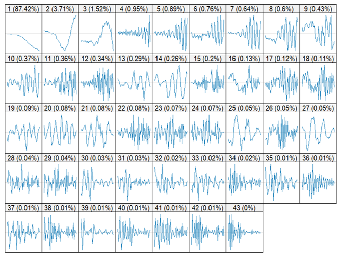
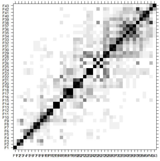
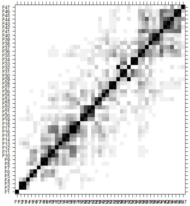
From Figure 4, it can be seen that the first component is a trend component that reflects data of 87.42% and the other component contains seasonal patterns. To see the similarity of characteristics more clearly, it can be seen with the help of the W-Correlation plot. The W-Correlation plot of Case 1 can be seen in Figure 5 below.
Figure 4. Eigentriple plot of Case 1
Figure 5. W-correlation plot of Case 1
The correlation of each component as visualized by Figure 5 can be found using Eq. (10) and the results can be seen in the following Table 6.
Table 6. W-correlation value of Case 1
|
Components |
F1 |
F2 |
F3 |
Fn |
F43 |
|
F1 |
1.000 |
0.116 |
0.067 |
$\cdots$ |
0.000 |
|
F2 |
0.116 |
1.000 |
0.577 |
$\cdots$ |
0.000 |
|
F3 |
0.067 |
0.577 |
1.000 |
$\cdots$ |
0.000 |
|
$\vdots$ |
$\vdots$ |
$\vdots$ |
$\vdots$ |
$\ddots$ |
$\vdots$ |
|
F43 |
0.000 |
0.000 |
0.000 |
$\cdots$ |
1.000 |
From Figure 5 and Table 6, it can be concluded that of the 43 components can be grouped into 18 groups based on the high and low correlation of each eigentriple. The height of the correlation can be seen based on the color of each component's slices, where the darker the correlation, the higher the correlation.
By using Eq. (11) and Eq. (12). The results of the diagonal averaging of the grouping stage can be seen in the following Table 7.
Table 7. Diagonal averaging Case 1
|
No. |
Diagonal Averaging |
|
1 |
-0.02 |
|
2 |
-0.59 |
|
3 |
-0.33 |
|
4 |
0.17 |
|
5 |
0.70 |
|
$\vdots$ |
$\vdots$ |
|
100 |
57.46 |
After the averaging diagonal calculation is obtained, then using the R-Forecasting method, namely Eqs. (14)-(16), forecasting can be calculated on the outsample data shown in Table 8.
3.2 Forecasting on Case 2
The insample data in Case 2 was converted into one-dimensional data as many as 106 data from 1900 to 2005 with the following arrangement:
$\left[\begin{array}{c}\text { Year 1900 } \\ \text { Year 1901 } \\ \text { Year 1902 } \\ \vdots \\ \text { Year 2005 }\end{array}\right]=\left[\begin{array}{c}x_1 \\ x_2 \\ x_3 \\ \vdots \\ x_{106}\end{array}\right]=\left[\begin{array}{c}0 \\ 0 \\ 0 \\ \vdots \\ 142\end{array}\right]$
After the data is converted into one dimension, then converted into multidimensional called the X trajectory matrix in L×K size. The optimal Windows Length (L) value is taken based on the smallest forecast accuracy value with a range of L values between 2≤L≤53, as shown in Table 9.
Table 8. SSA forecast results for Case 1
|
No. |
Year |
Current |
Predictions |
Difference |
|
1 |
2000 |
71 |
86.45 |
15.45 |
|
2 |
2001 |
60 |
111.27 |
51.27 |
|
3 |
2002 |
59 |
63.24 |
4.24 |
|
4 |
2003 |
81 |
82.87 |
1.87 |
|
5 |
2004 |
103 |
120.33 |
17.33 |
|
6 |
2005 |
142 |
131.83 |
10.17 |
|
7 |
2006 |
97 |
100.48 |
3.48 |
|
8 |
2007 |
115 |
149.30 |
34.30 |
|
9 |
2008 |
113 |
116.31 |
3.30 |
|
10 |
2009 |
76 |
150.29 |
74.29 |
|
11 |
2010 |
120 |
126.74 |
6.74 |
|
12 |
2011 |
110 |
178.61 |
68.61 |
|
13 |
2012 |
103 |
87.23 |
15.77 |
|
14 |
2013 |
127 |
94.10 |
32.90 |
|
15 |
2014 |
139 |
136.77 |
2.23 |
|
16 |
2015 |
122 |
140.46 |
18.46 |
|
17 |
2016 |
116 |
39.80 |
76.20 |
|
18 |
2017 |
112 |
134.79 |
22.79 |
|
19 |
2018 |
138 |
112.89 |
25.11 |
|
20 |
2019 |
134 |
78.13 |
55.87 |
|
21 |
2020 |
121 |
26.43 |
94.57 |
|
22 |
2021 |
123 |
232.35 |
109.35 |
|
23 |
2022 |
128 |
86.42 |
41.58 |
|
24 |
2023 |
98 |
96.86 |
1.14 |
|
RMSE |
45.25 |
|||
|
MAAPE |
1.43 |
|||
Table 9. Recapitulation of the results of measuring the level of forecast accuracy for Case 2
|
L |
Insample |
Outsample |
Normality |
Residual Independence |
||
|
RMSE |
MAAPE |
RMSE |
MAAPE |
|||
|
5 |
5.79 |
1.48 |
219.21 |
1.55 |
0 |
0.33 |
|
10 |
6.65 |
1.50 |
105.10 |
1.46 |
0 |
0.70 |
|
15 |
7.25 |
1.46 |
72.95 |
1.43 |
0 |
0.15 |
|
20 |
1.37 |
1.34 |
122.49 |
1.53 |
0 |
0.48 |
|
25 |
6.76 |
1.52 |
103.96 |
1.48 |
0 |
0.49 |
|
30 |
0.86 |
1.25 |
74.71 |
1.46 |
0.37 |
0.55 |
|
35 |
0.97 |
1.28 |
67.45 |
1.53 |
0.40 |
0.86 |
|
40 |
0.88 |
1.24 |
63.32 |
1.52 |
0.49 |
0.35 |
|
45 |
0.84 |
1.23 |
62.78 |
1.52 |
0.35 |
0.40 |
|
50 |
0.79 |
1.21 |
59.77 |
1.43 |
0.28 |
0.34 |
Obtained L with the minimum accuracy is 50. So, in the same way, tracking is carried out again around the values of 45 and 53 to get the most appropriate L value. It can be seen in the following Table 10.
As shown in Table 10, L=46 is printed in bold which indicates that the L value is the optimum L value because it has the smallest average accuracy value. Therefore, from the L value obtained, the value of K=61 is produced based on the equation K=N-L+1 where the value N=106.
Table 10. Forecasting accuracy of advanced Case 2
|
L |
Insample |
Outsample |
Normality |
Residual Independence |
||
|
RMSE |
MAAPE |
RMSE |
MAAPE |
|||
|
46 |
0.95 |
1.24 |
51.73 |
1.46 |
0.45 |
0.99 |
|
47 |
0.96 |
1.25 |
52.26 |
1.46 |
0.41 |
0.92 |
|
48 |
0.97 |
1.25 |
51.93 |
1.46 |
0.45 |
0.84 |
|
49 |
1.04 |
1.27 |
52.07 |
1.46 |
0.31 |
0.50 |
|
50 |
0.79 |
1.21 |
59.77 |
1.43 |
0.28 |
0.34 |
|
51 |
1.00 |
1.25 |
51.75 |
1.37 |
0.23 |
0.69 |
|
52 |
0.92 |
1.24 |
86.29 |
1.50 |
0.12 |
0.35 |
|
53 |
1.17 |
1.33 |
96.55 |
1.55 |
0.35 |
0.07 |
Furthermore, the process of forming the X trajectory matrix is by means that the values $x_1$ to $x_{46}$ become the first column, the values $x_2$ to $x_{47}$ become the second column, and so on until the values $x_{61}$ to $x_{106}$ become the 61 st column in the X trajectory matrix as written below:
$\boldsymbol{X}=\left[\begin{array}{cccccc}0 & 0 & 0 & 0 & \cdots & 1 \\ 0 & 0 & 0 & 0 & \cdots & 2 \\ \vdots & \vdots & \vdots & \vdots & \cdots & \vdots \\ 2 & 3 & 1 & 1 & \cdots & 142\end{array}\right]$
Next, the search for singular value, eigenvector, and principal component values will be carried out based on the trajectory matrix $X_{(46 \times 61)}$ that has been obtained in the previous stage. The first step is to create a symmetrical matrix as follows:
$\boldsymbol{S}=\boldsymbol{X} \boldsymbol{X}^{\boldsymbol{T}}=\boldsymbol{X}_{(46 \times 61)} \times \boldsymbol{X}_{(61 \times 46)}^T$
$\boldsymbol{S}=\left[\begin{array}{cccc}592 & 468 & \ldots & 4648 \\ 468 & 596 & \ldots & 4513 \\ \vdots & \vdots & \ddots & \vdots \\ 4648 & 4513 & \ldots & 89672\end{array}\right]$
After obtaining the symmetrical matrix $\boldsymbol{S}_{(46 \times 46)}$, then the singular value, eigenvector, and principal component (eigentriple) values will be searched for which satisfies, the eigentriple search is carried out by calculating the eigenvalue value, which then from eigenvalue can be calculated the singular value values by using Eq. (2) and Eq. (3) whose results are presented in Table 11 as follows:
Table 11. Eigenvalue and singular values of Case 2
|
No. |
Eigenvalue |
Singular Value |
|
1 |
724596.48 |
851.23 |
|
2 |
20465.51 |
143.06 |
|
3 |
16372.70 |
127.96 |
|
$\vdots$ |
$\vdots$ |
$\vdots$ |
|
46 |
18.47 |
4.30 |
Table 12. Eigenvector value of Case 2
|
No. |
U1 |
U2 |
U3 |
U$\cdots$ |
U46 |
|
1 |
-0.02 |
-0.05 |
-0.03 |
$\cdots$ |
0.29 |
|
2 |
-0.02 |
-0.05 |
-0.03 |
$\cdots$ |
-0.46 |
|
3 |
-0.02 |
-0.05 |
-0.02 |
$\cdots$ |
0.29 |
|
$\vdots$ |
$\vdots$ |
$\vdots$ |
$\vdots$ |
$\ddots$ |
$\vdots$ |
|
46 |
-0.34 |
-0.11 |
-0.54 |
$\cdots$ |
0.00 |
After the singular value is obtained, then find the eigenvector value of the symmetrical matrix $\boldsymbol{S}_{(46 \times 46)}$ using Eq. (2) which can be seen in Table 12.
After obtaining the eigenvalue and eigenvector values, then look for the principal component value by using Eq. (4) whose results are shown in the following Table 13.
Table 13. Principle component value of Case 2
|
No. |
V1 |
V2 |
V3 |
V$\cdots$ |
V46 |
|
1 |
-0.02 |
0.02 |
0.04 |
$\cdots$ |
0.01 |
|
2 |
-0.02 |
0.03 |
0.04 |
$\cdots$ |
-0.00 |
|
3 |
-0.02 |
0.03 |
0.04 |
$\cdots$ |
0.11 |
|
$\vdots$ |
$\vdots$ |
$\vdots$ |
$\vdots$ |
$\ddots$ |
$\vdots$ |
|
61 |
-0.34 |
0.08 |
-0.54 |
$\cdots$ |
-0.07 |
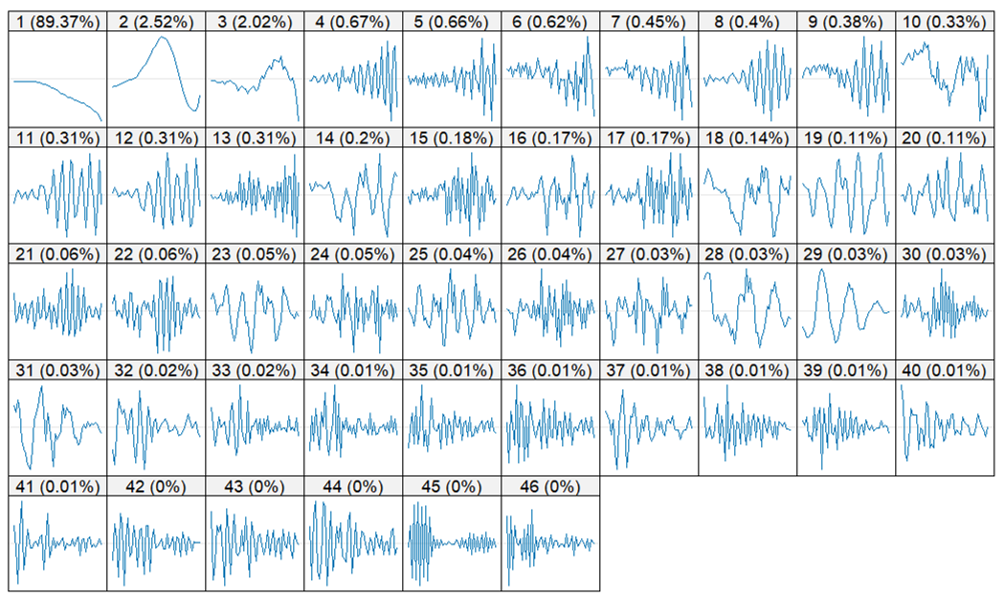
Furthermore, the data reconstruction from the results of the SVD calculation by grouping and diagonal averaging is carried out by grouping the eigentriple obtained from the SVD results according to the characteristics of each component. The selection of group members can be done by looking at the plot of the eigentriple. The following is shown the plot of each eigentriple with the value of i=1, 2, 3, ..., 46.
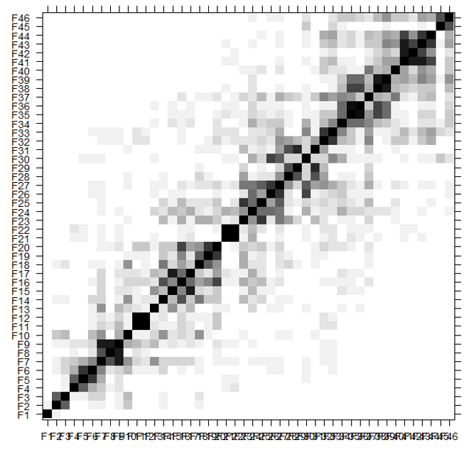
From Figure 6, it can be seen that the first component is a trend component that reflects data of 89.37% and the other component contains seasonal patterns. Grouping that is done by looking at plots from eigentriple is subjective. So there are several data patterns whose characteristics are difficult to distinguish. The W-Correlation plot of Case 2 can be seen in Figure 7 below.
Figure 6. Eigentriple plot of Case 2
Figure 7. W-correlation plot of Case 2
The correlation of each component as visualized by Figure 7 can be found using Eq. (10) and the results can be seen in the following Table 14.
Table 14. W-correlation value of Case 2
|
Components |
F1 |
F2 |
F3 |
Fn |
F46 |
|
F1 |
1.000 |
0.074 |
0.049 |
$\cdots$ |
0.000 |
|
F2 |
0.074 |
1.000 |
0.635 |
$\cdots$ |
0.000 |
|
F3 |
0.049 |
0.635 |
1.000 |
$\cdots$ |
-0.001 |
|
$\vdots$ |
$\vdots$ |
$\vdots$ |
$\vdots$ |
$\ddots$ |
$\vdots$ |
|
F46 |
0.000 |
0.000 |
-0.001 |
$\cdots$ |
1.000 |
Table 15. Diagonal averaging Case 2
|
No. |
Diagonal Averaging |
|
1 |
0.18 |
|
2 |
-0.70 |
|
3 |
-0.60 |
|
4 |
0.29 |
|
5 |
0.69 |
|
$\vdots$ |
$\vdots$ |
|
106 |
141.65 |
From Figure 7 and Table 14, it can be concluded that the 46 components can be grouped into 20 groups based on the high and low correlation of each eigentriple. The height of the correlation can be seen based on the color of each component's slices. where the darker the correlation, the higher the correlation.
By using Eq. (11) and Eq. (12), the results of the diagonal averaging of the grouping stage can be seen in Table 15.
After the averaging diagonal calculation is obtained, then using the R-Forecasting method, namely Eqs. (14)-(16). the forecast can be calculated on the outsample data shown in Table 16 below:
Table 16. SSA forecast results for Case 2
|
No. |
Year |
Actual |
Predictions |
Difference |
|
1 |
2006 |
97 |
43.84 |
53.16 |
|
2 |
2007 |
115 |
128.16 |
13.16 |
|
3 |
2008 |
113 |
97.16 |
15.84 |
|
4 |
2009 |
76 |
92.46 |
16.46 |
|
5 |
2010 |
120 |
121.88 |
1.88 |
|
6 |
2011 |
110 |
118.93 |
8.93 |
|
7 |
2012 |
103 |
93.95 |
9.04 |
|
8 |
2013 |
127 |
122.91 |
4.09 |
|
9 |
2014 |
139 |
100.56 |
38.44 |
|
10 |
2015 |
122 |
161.16 |
39.16 |
|
11 |
2016 |
116 |
19.60 |
96.40 |
|
12 |
2017 |
112 |
151.52 |
39.52 |
|
13 |
2018 |
138 |
120.18 |
17.82 |
|
14 |
2019 |
134 |
43.91 |
90.09 |
|
15 |
2020 |
121 |
92.28 |
28.72 |
|
16 |
2021 |
123 |
229.29 |
106.29 |
|
17 |
2022 |
128 |
125.06 |
2.94 |
|
18 |
2023 |
98 |
198.12 |
100.12 |
|
RMSE |
51.72 |
|||
|
MAAPE |
1.46 |
|||
3.3 Forecasting on Case 3
The insample data in Case 3 was converted into one-dimensional data as many as 112 data from 1900 to 2011 with the following arrangement:
$\left[\begin{array}{c}\text { Year 1900 } \\ \text { Year 1901 } \\ \text { Year 1902 } \\ \vdots \\ \text { Year 2011 }\end{array}\right]=\left[\begin{array}{c}x_1 \\ x_2 \\ x_3 \\ \vdots \\ x_{112}\end{array}\right]=\left[\begin{array}{c}0 \\ 0 \\ 0 \\ \vdots \\ 110\end{array}\right]$
After the data is converted into one dimension, then converted into multidimensional called the X trajectory matrix measuring L×K. The optimal Windows Length (L) value is taken based on the smallest forecast accuracy value with a value range of L between 2≤L≤55, using the grid method by trying the L values of 5, 10, 15, 20, 25, 30, 35, 40, 45, 50, 55. as shown in Table 17.
Table 17. Recapitulation of the results of measuring the level of forecast accuracy for Case 3
|
L |
Insample |
Outsample |
Normality |
Residual Independence |
||
|
RMSE |
MAAPE |
RMSE |
MAAPE |
|||
|
5 |
3.41 |
1.42 |
28.57 |
1.34 |
0 |
0 |
|
10 |
4.18 |
1.43 |
79.62 |
1.52 |
0 |
0.01 |
|
15 |
3.58 |
1.44 |
49.37 |
1.46 |
0 |
0.56 |
|
20 |
3.18 |
1.42 |
45.64 |
1.37 |
0 |
0.28 |
|
25 |
1.66 |
1.35 |
82.16 |
1.52 |
0 |
0.01 |
|
30 |
3.26 |
1.43 |
55.37 |
1.51 |
0 |
0.12 |
|
35 |
2.75 |
1.43 |
53.80 |
1.51 |
0 |
0.06 |
|
40 |
1.16 |
1.28 |
64.81 |
1.52 |
0.74 |
0.36 |
|
45 |
1.02 |
1.26 |
60.47 |
1.53 |
0.56 |
0.29 |
|
50 |
0.91 |
1.19 |
58.67 |
1.53 |
0.30 |
0.29 |
|
55 |
0.94 |
1.19 |
80.49 |
1.42 |
0.09 |
0.04 |
In Table 17, L with values of 5, 10, 15, 20, 25, 30, and 35 has abnormal residuals because the p-value obtained is less than α=0.05. Therefore, L is obtained with the minimum accuracy of 50. So, in the same way, tracking is carried out again around the values of 45 and 55 to get the most appropriate L value. It can be seen in Table 18 below:
Table 18. Forecasting accuracy of advanced Case 3
|
L |
Insample |
Outsample |
Normality |
Residual Independence |
||
|
RMSE |
MAAPE |
RMSE |
MAAPE |
|||
|
46 |
0.86 |
1.17 |
56.56 |
1.50 |
0.69 |
0.57 |
|
47 |
0.88 |
1.18 |
55.25 |
1.53 |
0.73 |
0.54 |
|
48 |
0.89 |
1.18 |
55.94 |
1.47 |
0.66 |
0.44 |
|
49 |
0.90 |
1.19 |
56.59 |
1.52 |
0.43 |
0.35 |
|
50 |
0.91 |
1.19 |
58.67 |
1.53 |
0.30 |
0.29 |
|
51 |
0.84 |
1.16 |
60.41 |
1.48 |
0.09 |
0.18 |
|
52 |
0.86 |
1.16 |
61.07 |
1.40 |
0.08 |
0.15 |
|
53 |
0.83 |
1.13 |
57.67 |
1.51 |
0.06 |
0.24 |
|
54 |
0.89 |
1.16 |
62.65 |
1.51 |
0.05 |
0.10 |
As shown in Table 18, L=47 is printed in bold which indicates that the L value is the optimal L value because it has the smallest average accuracy value. Therefore, from the value of L obtained, the value of K=66 is based on the equation K=N-L+1 where the value of N=112. Furthermore, the process of forming the X trajectory matrix is by means that the values $x_1$ to $x_{47}$ become the first column, the values $x_2$ to $x_{48}$ become the second column and so on until the values $x_{66}$ to $x_{112}$ become the 66th column in the X trajectory matrix as written as follows:
$\boldsymbol{X}=\left[\begin{array}{cccccc}0 & 0 & 0 & 0 & \cdots & 6 \\ 0 & 0 & 0 & 0 & \cdots & 1 \\ \vdots & \vdots & \vdots & \vdots & \cdots & \vdots \\ 3 & 1 & 1 & 4 & \cdots & 110\end{array}\right]$
Next, the search for singular value, eigenvector, and principal component values is carried out based on the trajectory matrix $\boldsymbol{X}_{(47 \times 66)}$ that has been obtained in the previous stage. The first step is to create a symmetrical matrix as follows:
$\boldsymbol{S}=\left[\begin{array}{cccc}694 & 542 & \ldots & 7070 \\ 542 & 695 & \ldots & 6845 \\ \vdots & \vdots & \ddots & \vdots \\ 7070 & 6845 & \ldots & 157347\end{array}\right]$
After obtaining the symmetrical matrix $\boldsymbol{S}_{(47 \times 47)}$, then the singular value, eigenvector, and principal component (eigentriple) values will be searched that meet, the eigentriple search is carried out by calculating the eigenvalue value, which then from eigenvalue can be calculated the singular values by using Eq. (2) and Eq. (3) whose results are presented in Table 19 as follows:
Table 19. Eigenvalue and singular value of Case 3
|
No. |
Eigenvalue |
Singular Value |
|
1 |
1444133 |
1201.72 |
|
2 |
24829.94 |
157.58 |
|
3 |
21120.39 |
145.33 |
|
$\vdots$ |
$\vdots$ |
$\vdots$ |
|
47 |
22.33 |
4.73 |
After the singular value is obtained, then find the eigenvector value of the symmetric matrix $\boldsymbol{S}_{(47 \times 47)}$ using Eq. (2) whose results can be seen in Table 20 as follows.
Table 20. Eigenvector value of Case 3
|
No. |
U1 |
U2 |
U3 |
U$\cdots$ |
U47 |
|
1 |
-0.01 |
0.02 |
-0.04 |
$\cdots$ |
-0.13 |
|
2 |
-0.01 |
0.02 |
-0.03 |
$\cdots$ |
0.22 |
|
3 |
-0.02 |
0.03 |
-0.03 |
$\cdots$ |
-0.26 |
|
$\vdots$ |
$\vdots$ |
$\vdots$ |
$\vdots$ |
$\ddots$ |
$\vdots$ |
|
47 |
-0.32 |
0.15 |
0.17 |
$\cdots$ |
0.03 |
After obtaining the eigenvalue and eigenvector values, then find the principal component value by using Eq. (4) which is the result in Table 21.
Furthermore, the data reconstruction from the results of the SVD calculation by grouping and diagonal averaging by grouping the eigentriple obtained from the SVD results according to the characteristics of each component. The selection of group members can be done by looking at the plot of the eigentriple.
Table 21. Principle component value of Case 3
|
No. |
V1 |
V2 |
V3 |
V$\cdots$ |
V47 |
|
1 |
-0.01 |
-0.04 |
-0.01 |
$\cdots$ |
0.18 |
|
2 |
-0.01 |
-0.04 |
-0.00 |
$\cdots$ |
-0.21 |
|
3 |
-0.01 |
-0.05 |
-0.00 |
$\cdots$ |
0.20 |
|
$\vdots$ |
$\vdots$ |
$\vdots$ |
$\vdots$ |
$\ddots$ |
$\vdots$ |
|
66 |
-0.32 |
0.16 |
-0.16 |
$\cdots$ |
0.01 |
Figure 8. Eigentriple plot Case 3
Figure 9. W-correlation plot of Case 3
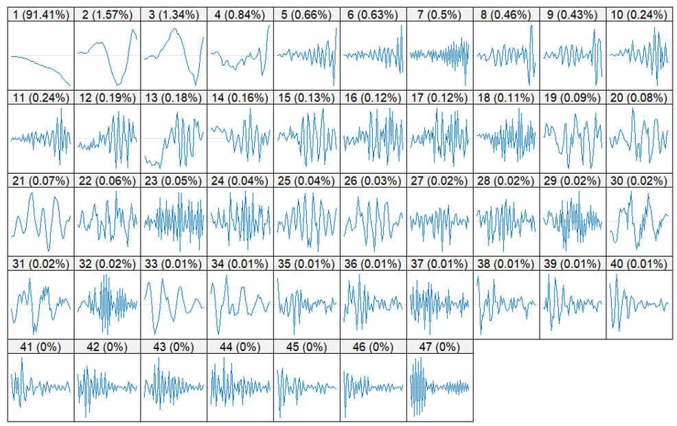
From Figure 8, it can be seen that the first component is a trend component that reflects data of 91,41% and the other component contains seasonal patterns. Grouping that is done by looking at plots from eigentriple is subjective. The W-Correlation plot of Case 3 can be seen in Figure 9.
The correlation of each component as visualized by Figure 10 can be searched using Eq. (10) and the results can be seen in the following Table 22.
Table 22. W-correlation value of Case 3
|
Components |
F1 |
F2 |
F3 |
Fn |
F47 |
|
F1 |
1.000 |
0.038 |
0.042 |
$\cdots$ |
0.000 |
|
F2 |
0.038 |
1.000 |
0.937 |
$\cdots$ |
0.000 |
|
F3 |
0.042 |
0.937 |
1.000 |
$\cdots$ |
0.000 |
|
$\vdots$ |
$\vdots$ |
$\vdots$ |
$\vdots$ |
$\ddots$ |
$\vdots$ |
|
F47 |
0.000 |
0.000 |
0.000 |
$\cdots$ |
1.000 |
From Figure 9 and Table 22, it can be concluded that the 47 components can be grouped into 23 groups based on the high and low correlation of each eigentriple. The height of the correlation can be seen based on the color of each component's slices, where the darker the correlation, the higher the correlation. Using Eq. (11) and Eq. (12), the diagonal averaging results of the grouping stage can be seen in Table 23.
Table 23. Diagonal averaging Case 3
|
No. |
Diagonal Averaging |
|
1 |
0.19 |
|
2 |
-0.69 |
|
3 |
-0.66 |
|
4 |
0.34 |
|
5 |
0.60 |
|
$\vdots$ |
$\vdots$ |
|
112 |
109.83 |
Table 24. SSA forecast results for Case 3
|
No. |
Year |
Actual |
Prediction |
Difference |
|
1 |
2012 |
103 |
88.69 |
14.31 |
|
2 |
2013 |
127 |
177.13 |
50.13 |
|
3 |
2014 |
139 |
164.42 |
25.42 |
|
4 |
2015 |
122 |
105.37 |
16.63 |
|
5 |
2016 |
116 |
80.17 |
35.83 |
|
6 |
2017 |
112 |
49.19 |
62.81 |
|
7 |
2018 |
138 |
77.81 |
60.19 |
|
8 |
2019 |
134 |
54.60 |
79.40 |
|
9 |
2020 |
121 |
79.73 |
41.27 |
|
10 |
2021 |
123 |
244.07 |
121.07 |
|
11 |
2022 |
128 |
143.18 |
15.18 |
|
12 |
2023 |
98 |
133.25 |
35.25 |
|
RMSE |
55.25 |
|||
|
MAAPE |
1.53 |
|||
After the diagonal averaging calculation is obtained, then using the R-Forecasting method, namely Eq. (14), Eq. (15), and Eq. (16), the forecast can be calculated on the outsample data shown in Table 24.
3.4 Forecasting on Case 4
The insample data in Case 4 was converted into one-dimensional data of 118 data from 1900 to 2017 with the following arrangement.
$\left[\begin{array}{c}\text { Year 1900 } \\ \text { Year 1901 } \\ \text { Year 1902 } \\ \vdots \\ \text { Year 2017 }\end{array}\right]=\left[\begin{array}{c}x_1 \\ x_2 \\ x_3 \\ \vdots \\ x_{118}\end{array}\right]=\left[\begin{array}{c}0 \\ 0 \\ 0 \\ \vdots \\ 112\end{array}\right]$
After the data is converted into one dimension, then converted into multidimensional called an X trajectory matrix measuring L×K. The optimal Windows Length (L) value is taken based on the smallest forecast accuracy value with a value range of L between 2≤L≤55, using the grid method by trying the L values, as shown in Table 25.
Table 25. Recapitulation of the results of measuring the level of forecast accuracy for Case 4
|
L |
Insample |
Outsample |
Normality |
Residual Independence |
||
|
RMSE |
MAAPE |
RMSE |
MAAPE |
|||
|
5 |
7.29 |
1.49 |
31.16 |
1.34 |
0 |
0.09 |
|
10 |
4.29 |
1.43 |
37.05 |
1.53 |
0 |
0 |
|
15 |
4.55 |
1.44 |
32.79 |
1.52 |
0 |
0 |
|
20 |
4.84 |
1.45 |
65.52 |
1.52 |
0 |
0.02 |
|
25 |
3.87 |
1.46 |
50.40 |
1.33 |
0 |
0.01 |
|
30 |
1.01 |
1.24 |
40.48 |
1.46 |
0.09 |
0.79 |
|
35 |
1.47 |
1.30 |
55.00 |
1.46 |
0.08 |
0.05 |
|
40 |
1.49 |
1.30 |
95.87 |
1.54 |
0.11 |
0.22 |
|
45 |
1.12 |
1.24 |
59.12 |
1.52 |
0.64 |
0.97 |
|
50 |
0.96 |
1.16 |
36.04 |
1.51 |
0.34 |
0.20 |
|
55 |
1.10 |
1.22 |
25.48 |
1.48 |
0.25 |
0.32 |
Table 26. Forecasting accuracy of advanced Case 4
|
L |
Insample |
Outsample |
Normality |
Residual Independence |
||
|
RMSE |
MAAPE |
RMSE |
MAAPE |
|||
|
51 |
1.06 |
1.22 |
29.65 |
1.41 |
0.35 |
0.85 |
|
52 |
1.07 |
1.23 |
28.83 |
1.44 |
0.30 |
0.58 |
|
53 |
1.08 |
1.23 |
25.67 |
1.29 |
0.25 |
0.44 |
|
54 |
1.10 |
1.22 |
25.48 |
1.48 |
0.25 |
0.32 |
|
55 |
1.10 |
1.22 |
25.48 |
1.48 |
0.25 |
0.32 |
|
56 |
1.12 |
1.23 |
25.15 |
1.49 |
0.25 |
0.18 |
|
57 |
1.13 |
1.22 |
25.23 |
1.43 |
0.26 |
0.10 |
|
58 |
1.14 |
1.23 |
25.94 |
1.46 |
0.27 |
0.07 |
|
59 |
1.15 |
1.23 |
29.92 |
1.44 |
0.28 |
0.06 |
In Table 25, L with values of 5, 10, 15, 20, and 25 has abnormal residuals because the p-value obtained is less than α=0.05. Therefore, obtained L with the minimum accuracy is 55. So, in the same way, tracking is carried out again around the value of 55 to get the most appropriate L value. It can be seen in Table 26.
As shown in Table 26, L=56 is bolded which indicates that the L value is the optimum L value because it has the smallest average accuracy value. Therefore, from the value of L obtained, the value of K=63 is produced based on the equation K=N-L+1 where the value of N=118. Furthermore, the process of forming the X trajectory matrix is by means that the values $x_1$ to $x_{56}$ become the first column, the values $x_2$ to $x_{57}$ become the second column and so on until the values $x_{63}$ to $x_{118}$ become the 63 rd column in the $\mathbf{X~}$trajectory matrix as written as follows:
$\boldsymbol{X}=\left[\begin{array}{cccccc}0 & 0 & 0 & 0 & \cdots & 1 \\ 0 & 0 & 0 & 0 & \cdots & 6 \\ \vdots & \vdots & \vdots & \vdots & \cdots & \vdots \\ 3 & 2 & 4 & 1 & \cdots & 112\end{array}\right]$
Next, the search for singular value, eigenvector, and principal component values will be carried out based on the trajectory matrix $\boldsymbol{X}_{(56 \times 63)}$ that has been obtained in the previous stage.
$\boldsymbol{S}=\left[\begin{array}{cccc}597 & 476 & \ldots & 8051 \\ 476 & 633 & \ldots & 8368 \\ \vdots & \vdots & \ddots & \vdots \\ 8051 & 8368 & \ldots & 244197\end{array}\right]$
After obtaining the symmetrical matrix $\boldsymbol{S}_{(56 \times 56)}$, then the singular value, eigenvector, and principal component (eigentriple) values will be searched that meet, the eigentriple search is carried out by calculating the eigenvalue value, then from eigenvalue the singular values can be calculated using Eq. (2) and Eq. (3) whose results are presented in Table 27.
Table 27. Eigenvalue and singular values of Case 4
|
No. |
Eigenvalue |
Singular Value |
|
1 |
2628656 |
1621.31 |
|
2 |
33154.67 |
182.08 |
|
3 |
24824.69 |
157.56 |
|
$\vdots$ |
$\vdots$ |
$\vdots$ |
|
56 |
11.43 |
3.38 |
After the singular value is obtained, then find the eigenvector value of the symmetric matrix $\boldsymbol{S}_{(56 \times 56)}$ using Eq. (2) whose results can be seen in Table 28.
Table 28. Eigenvector value of Case 4
|
No. |
U1 |
U2 |
U3 |
U$\cdots$ |
U56 |
|
1 |
-0.01 |
-0.01 |
-0.00 |
$\cdots$ |
0.38 |
|
2 |
-0.01 |
-0.01 |
-0.00 |
$\cdots$ |
-0.31 |
|
3 |
-0.01 |
-0.01 |
-0.01 |
$\cdots$ |
-0.16 |
|
$\vdots$ |
$\vdots$ |
$\vdots$ |
$\vdots$ |
$\ddots$ |
$\vdots$ |
|
56 |
-0.30 |
-0.40 |
-0.05 |
$\cdots$ |
-0.07 |
Table 29. Principle component value of Case 4
|
No. |
V1 |
V2 |
V3 |
V$\cdots$ |
V56 |
|
1 |
-0.01 |
-0.00 |
0.04 |
$\cdots$ |
-0.02 |
|
2 |
-0.01 |
-0.00 |
0.03 |
$\cdots$ |
-0.09 |
|
3 |
-0.01 |
-0.01 |
0.03 |
$\cdots$ |
-0.13 |
|
$\vdots$ |
$\vdots$ |
$\vdots$ |
$\vdots$ |
$\ddots$ |
$\vdots$ |
|
63 |
-0.30 |
0.40 |
0.06 |
$\cdots$ |
0.02 |
After obtaining the eigenvalue and eigenvector values, then find the principal component value by using Eq. (4) whose results are shown in Table 29.
Furthermore, the data reconstruction from the results of the SVD calculation was carried out by grouping and diagonal averaging which was carried out by grouping the eigentriple obtained from the SVD results according to the characteristics of each component. The selection of group members can be done by looking at the plot of the eigentriple. The following is shown the plot of each eigentriple with a value of i=1, 2, 3, ..., 56.
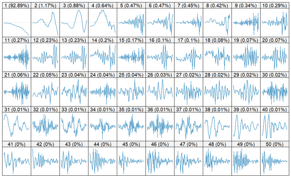
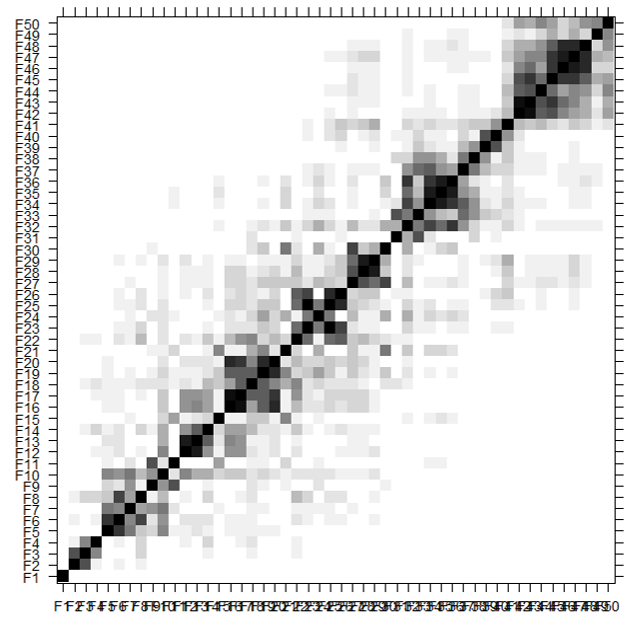
From Figure 10, it can be seen that the first component is a trend component that reflects data of 92.89% and the other component contains seasonal patterns (Only a maximum of 50 can be displayed). Grouping that is done by looking at plots from eigentriple is subjective. So there are several data patterns whose characteristics are difficult to distinguish. To see the similarity of characteristics more clearly, it can be seen with the help of the W-Correlation plot. The W-Correlation plot of Case 4 can be seen in Figure 11.
Figure 10. Eigentriple plot Case 4
Figure 11. W-correlation plot of Case 4
The correlation of each component as visualized by Figure 11 can be searched using Eq. (10) and the results can be seen in the following Table 30.
Table 30. W-correlation value of Case 4
|
Components |
F1 |
F2 |
F3 |
Fn |
F56 |
|
F1 |
1.000 |
0.029 |
0.032 |
$\cdots$ |
0.000 |
|
F2 |
0.029 |
1.000 |
0.676 |
$\cdots$ |
0.000 |
|
F3 |
0.032 |
0.676 |
1.000 |
$\cdots$ |
0.000 |
|
$\vdots$ |
$\vdots$ |
$\vdots$ |
$\vdots$ |
$\ddots$ |
$\vdots$ |
|
F56 |
0.000 |
0.000 |
0.000 |
$\cdots$ |
1.000 |
Table 31. Diagonal averaging Case 4
|
No. |
Diagonal Averaging |
|
1 |
0.44 |
|
2 |
-0.29 |
|
3 |
-0.24 |
|
4 |
0.41 |
|
5 |
0.54 |
|
$\vdots$ |
$\vdots$ |
|
118 |
111.63 |
Table 32. SSA forecast results for Case 4
|
No. |
Year |
Actual |
Prediction |
Difference |
|
1 |
2018 |
138 |
148.77 |
10.77 |
|
2 |
2019 |
134 |
94.74 |
39.26 |
|
3 |
2020 |
121 |
103.49 |
17.51 |
|
4 |
2021 |
123 |
161.48 |
38.48 |
|
5 |
2022 |
128 |
111.31 |
16.69 |
|
6 |
2023 |
98 |
89.59 |
8.41 |
|
RMSE |
25.15 |
|||
|
MAAPE |
1.49 |
|||
From Figure 8 and Table 30, it can be concluded that of the 56 components can be grouped into 23 groups based on the high and low correlation of each eigentriple. The height of the correlation can be seen based on the color of each component's slices, where the darker the correlation, the higher the correlation. The results of the diagonal averaging of the grouping stage can be seen in Table 31.
After the averaging diagonal calculation is obtained, then using the R-Forecasting method, the forecast can be calculated on the outsample data shown in Table 32 in the form of forecast results for the outsample data.
3.5 Discussion
The performance of SSA is evaluated using four different cases, each with varying proportions of training and testing data. The higher RMSE here reflects slightly larger deviations in predictions, particularly for testing years with higher seismic variability. However, MAAPE remains stable, emphasizing the model’s robustness in interpreting low actual values. For case 3, produced the highest RMSE, indicating more significant prediction errors. This could be attributed to the shorter test period capturing more recent seismic fluctuations. The slightly higher MAAPE also suggests challenges in maintaining angular prediction consistency for these years. Subsequently, for Case 4 (1900–2017 training, 2018–2023 testing): Case 4 achieved the lowest RMSE, demonstrating the highest predictive accuracy. This result suggests that the SSA model performed exceptionally well with a larger training set (spanning nearly the entire dataset) and a shorter test set. Although MAAPE is slightly higher than in case 1, the values still indicate reliable performance. Interpretation and Real-World Implications These results highlight the strengths and limitations of SSA across different data configurations. RMSE provides a granular understanding of the magnitude of prediction errors, emphasizing the importance of accurate forecasts in years with higher earthquake frequencies. Meanwhile, MAAPE underscores the reliability of the model in interpreting data with extreme values, a crucial feature for seismic hazard assessments in the Sumatra subduction zone. In practice, lower RMSE values, such as those observed for Case 4, are desirable as they signify better alignment between predictions and observed frequencies. However, MAAPE’s stability across all pairs confirms the SSA model’s robustness, even in scenarios with low earthquake frequencies or significant variability. This robustness ensures that SSA predictions can be trusted for real-world applications, such as disaster preparedness and resource allocation. By combining RMSE and MAAPE, this study not only assesses statistical performance but also links these metrics to practical considerations in seismic forecasting. The findings validate SSA’s capability to provide reliable earthquake frequency forecasts, thereby supporting efforts to mitigate risks and improve readiness in one of the world’s most seismically active regions.
The forecasting results of this study hold significant practical implications, particularly in supporting disaster risk management in the highly active Sumatra subduction zone. Accurate forecasts of earthquake frequency can improve the effectiveness of early warning systems by providing actionable insights into seismic trends. By understanding the likely frequency of earthquake events within a given time frame, authorities can enhance real-time monitoring systems and optimize their preparedness for potential earthquakes. This is particularly valuable in mitigating cascading effects, such as tsunamis, which often follow large-magnitude earthquakes in this region. For instance, the model’s ability to predict earthquake frequencies with low RMSE (as observed in Case 4) ensures a higher degree of confidence in early alerts, allowing communities in high-risk areas to evacuate in time and minimize loss of life. In addition, one of the critical challenges during seismic events is the efficient allocation of emergency resources, such as medical aid, search and rescue teams, and temporary shelters. Forecasting earthquake frequency enables disaster management agencies to identify periods of heightened seismic activity and allocate resources proactively. This reduces response times and enhances the overall effectiveness of emergency operations. For example, the predictive results for testing years (e.g., RMSE=25.15 for Case 4) could guide the pre-positioning of emergency supplies in regions with historically higher seismic activity, such as the Mentawai segment of the Sumatra subduction zone.
Our study’s critical analysis of cases explores the performance and implications of different in-sample and out-sample compositions in forecasting earthquake frequency using SSA. Four data configurations (80%-20%, 85%-15%, 90%-10%, and 95%-5%) were tested, revealing that Case 3 (90%-10%) offered the best balance, achieving the lowest RMSE and MAAPE for in-sample predictions. This optimal balance ensured reliable forecasts without sacrificing adaptability, while larger training sets like Case 4 (95%-5%) enhanced out-sample accuracy but struggled with recent seismic fluctuations. Notably, MAAPE’s stability across all cases underscored SSA’s reliability in handling data variability and extreme events. These findings have significant real-world implications, particularly for seismic hazard assessments in the Sumatra subduction zone. Improved predictive accuracy supports early warning systems, enabling timely evacuations and proactive resource allocation in high-risk areas like the Mentawai segment. The low RMSE achieved in testing years exemplifies the SSA model’s potential to align closely with observed earthquake patterns, providing actionable insights for disaster preparedness. This analysis validates SSA’s robustness and utility, offering a foundation for further integration with advanced techniques to enhance forecasting methodologies and risk mitigation strategies.
This study acknowledges several limitations of the SSA approach for earthquake frequency forecasting in the Sumatra subduction zone. One notable challenge is the risk of overfitting, particularly with configurations that utilize high in-sample percentages, such as Case 4 (95%-5%). While this configuration improves in-sample predictive accuracy, it can reduce the model's ability to generalize effectively to unseen data. To address this, balanced data splits and robust cross-validation methods are essential to enhance model reliability and applicability. Additionally, predicting extreme seismic events, such as megathrust earthquakes, presents significant difficulties. These rare, high-impact events often deviate from the historical patterns captured by time-series models like SSA, limiting the model’s effectiveness in these scenarios. To overcome these challenges, future research should focus on integrating SSA with advanced techniques such as machine learning models, which can leverage complex patterns from large datasets. Incorporating geophysical data, including tectonic stress distributions and surface deformation measurements, could further enhance the model’s predictive power. Expanding the application of this approach to other tectonic regions would also test its generalizability and provide comparative insights. By addressing these limitations, future efforts can refine SSA-based forecasting, ensuring its robustness in capturing both routine seismic patterns and rare, extreme events. These advancements hold the potential to improve disaster risk management and preparedness in earthquake-prone regions.
This study demonstrates that SSA is an effective method for modeling and predicting earthquake frequency in the Sumatra subduction zone, a region with significant tectonic activity. The findings highlight SSA’s ability to analyze complex, non-linear, and non-stationary time series data, offering a novel approach to earthquake forecasting. A key contribution of this research lies in its comprehensive evaluation of four different insample-outsample data splits, which revealed that a 90% insample and 10% outsample composition provided the best performance for insample predictions. Additionally, the study underscores the practical relevance of SSA in addressing disaster preparedness in one of the world's most hazardous seismic zones. However, the reliability of SSA depends heavily on the availability of high-quality historical data, and its ability to forecast extreme events, such as megathrust earthquakes, remains uncertain due to the complexity of tectonic dynamics.
Future research could enhance SSA’s predictive capabilities by integrating it with techniques such as Machine Learning or statistical models like ARIMA or GARCH, applying it to other seismic regions to test its generalizability, and incorporating additional geophysical data such as tectonic stress or surface deformation. These advancements could broaden the applicability of SSA in disaster mitigation and improve preparedness in earthquake-prone regions.
This work was supported by the Faculty of Mathematics and Natural Sciences (FMIPA), University of Bengkulu, Indonesia, through “Penelitian Unggulan FMIPA 2024” (Grant numbers: 2687/UN30.12/HK/2024).
[1] Sieh, K., Natawidjaja, D. (2000). Neotectonics of the Sumatran fault, Indonesia. Journal of Geophysical Research: Solid Earth, 105(B12): 28295-28326. https://doi.org/10.1029/2000JB900120
[2] Irsyam, M., Cummins, P.R., Asrurifak, M., Faizal, L., Natawidjaja, D.H., Widiyantoro, S., Meilano, I., Triyoso, W., Rudiyanto, A., Hidayati, S., Ridwan, M., Hanifa, N. R., Syahbana, A.J. (2020). Development of the 2017 national seismic hazard maps of Indonesia. Earthquake Spectra, 36(1_suppl): 112-136. https://doi.org/10.1177/8755293020951206
[3] Rizal, J., Gunawan, A.Y., Yosmar, S., Nuryaman, A. (2024). Seismicity pattern recognition in the Sumatra megathrust zone through mathematical modeling of the maximum earthquake magnitude using gaussian mixture models. Mathematical Modelling of Engineering Problems, 11(5): 1179-1188. https://doi.org/10.18280/mmep.110506
[4] Helmstetter, A., Sornette, D., Grasso, J.R. (2006). Mainshocks are aftershocks of conditional foreshocks: How do foreshock statistical properties emerge from aftershock laws. Journal of Geophysical Research: Solid Earth, 111(B5). https://doi.org/10.1029/2002JB001991
[5] Luen, B., Stark, P.B. (2012). Poisson tests of declustered catalogues. Geophysical Journal International, 189(1): 691-700. https://doi.org/10.1111/j.1365-246X.2012.05400.x
[6] Zhigljavsky, A. (2010). Singular Spectrum Analysis for time series: Introduction to this special issue. Statistics and Its Interface, 3(3): 255-258. https://doi.org/10.4310/SII.2010.v3.n3.a1
[7] Wang, R., Ma, H.G., Qin, J.Q., Feng, X.W., Liu, H.M. (2015). Analysis of death series by SSA based BSS technique. In 2015 10th International Conference on Information, Communications and Signal Processing (ICICS), Singapore, pp. 1-5. https://doi.org/10.1109/ICICS.2015.7459854
[8] Golyandina, N., Zhigljavsky, A. (2020). Singular Spectrum Analysis for Time Series. SpringerBriefs in Statistics. https://doi.org/10.1007/978-3-662-62436-4
[9] Leles, M.C., Sansão, J.P.H., Mozelli, L.A., Guimarães, H.N. (2018). Improving reconstruction of time-series based in Singular Spectrum Analysis: A segmentation approach. Digital Signal Processing, 77: 63-76. https://doi.org/10.1016/j.dsp.2017.10.025
[10] Trendafilova, I. (2021). Singular Spectrum Analysis for the investigation of structural vibrations. Engineering Structures, 242: 112531. https://doi.org/10.1016/j.engstruct.2021.112531
[11] Mukhopadhyay, S.K., Krishnan, S. (2020). A Singular Spectrum Analysis-based model-free electrocardiogram denoising technique. Computer Methods and Programs in Biomedicine, 188: 105304. https://doi.org/10.1016/j.cmpb.2019.105304
[12] Kalantari, M., Hassani, H. (2019). Automatic grouping in Singular Spectrum Analysis. Forecasting, 1(1): 189-204. https://doi.org/10.3390/forecast1010013
[13] Rodrigues, P.C., Lourenço, V., Mahmoudvand, R. (2018). A robust approach to Singular Spectrum Analysis. Quality and Reliability Engineering International, 34(7): 1437-1447. https://doi.org/10.1002/qre.2337
[14] Leles, M.C., Sansão, J.P.H., Mozelli, L.A., Guimarães, H.N. (2018). A new algorithm in Singular Spectrum Analysis framework: The Overlap-SSA (ov-SSA). SoftwareX, 8: 26-32. https://doi.org/10.1016/j.softx.2017.11.001
[15] Golub, G.H., Van der Vorst, H.A. (2000). Eigenvalue computation in the 20th century. Journal of Computational and Applied Mathematics, 123(1-2): 35-65. https://doi.org/10.1016/S0377-0427(00)00413-1
[16] Trefethen, L.N., David Bau, III. (1997). Numerical linear algebra. Philadelphia: Society for Industrial and Applied Mathematics. https://doi.org/10.1137/1.9780898719574
[17] Meyer, C.D. (2000). Matrix analysis and applied linear algebra. Society for Industrial and Applied Mathematics. https://doi.org/10.4236/oalib.1108330
[18] Sulandari, W., Subanar, S., Lee, M.H., Rodrigues, P.C. (2020). Time series forecasting using Singular Spectrum Analysis, fuzzy systems and neural networks. MethodsX, 7: 101015. https://doi.org/10.1016/j.mex.2020.101015
[19] Asrof, A., Ischack, R., Darmawan, G. (2017). Forecasting red chili production in West Java using the Singular Spectrum Analysis (SSA) method. Statistics, 17(2): 77-87. http://doi.org/10.29313/jstat.v17i2.2839
[20] Koutsandreas, D., Spiliotis, E., Petropoulos, F., Assimakopoulos, V. (2022). On the selection of forecasting accuracy measures. Journal of the Operational Research Society, 73(5): 937-954. https://doi.org/10.1080/01605682.2021.1892464
[21] Lin, S.L., Huang, H.W. (2020). Improving deep learning for forecasting accuracy in financial data. Discrete Dynamics in Nature and Society, 2020(1): 5803407. https://doi.org/10.1155/2020/5803407
[22] Estrada, M.D.R.C., Camarillo, M.E.G., Parraguirre, M.E.S., Edgar, M., Castillo, G., Juárez, E.M., Gómez, M.J.C. (2020). Evaluation of several error measures applied to the sales forecast system of chemicals supply enterprises. International Journal of Business Administration, 11(4): 39-51. https://doi:10.5430/ijba.v11n4p39
[23] Mahan, M.Y., Chorn, C.R., and Georgopoulos, A.P. (2015). White noise test: Detecting autocorrelation and nonstationarities in long time series after ARIMA modeling. In SciPy Proceedings, pp. 97-104. https://doi.org/10.25080/Majora-7b98e3ed-00f
[24] Kwak, S.G., Park, S.H. (2019). Normality test in clinical research. Journal of Rheumatic Diseases, 26(1): 5-11. https://doi.org/10.4078/jrd.2019.26.1.5
[25] Jäntschi, L., Bolboacă, S.D. (2018). Computation of probability associated with Anderson-Darling statistic. Mathematics, 6(6): 88. https://doi.org/10.3390/math6060088