Sigit Susanto Putro*![]() | Nachnul Ansori
| Nachnul Ansori![]() | Muhammad Fuad
| Muhammad Fuad![]() | Eka Mala Sari Rochman
| Eka Mala Sari Rochman![]() | Yuli Panca Asmara
| Yuli Panca Asmara![]() | Aeri Rachmad
| Aeri Rachmad![]()
© 2025 The authors. This article is published by IIETA and is licensed under the CC BY 4.0 license (http://creativecommons.org/licenses/by/4.0/).
OPEN ACCESS
Corn is an important cereal crop that ranks third as a global food necessity after rice and wheat, and it is a primary source of carbohydrates in Indonesia after rice. The varied products of corn, including animal feed and industrial raw materials, make it a high-value commodity. However, corn food productivity is often disrupted by diseases such as leaf rust and leaf blight, which can significantly reduce yields. To overcome this problem, this research aims to increase food productivity by looking for a combination model of Convolutional Neural Network (CNN) Model with Optimizer and Batch Size in identifying diseases on corn leaves. This study uses the MobileNetV2 CNN architecture to classify images of disease corn leaf. Adam and RMSProp optimization parameters equipped with predetermined learning rates were utilized in this study for training and testing data divided into 70% and 30% respectively. Test results show a significant increase in accuracy, precision, recall, and F1 score over training epochs. The test results of the CNN model with MobileNetV2 architecture with a learning rate of 0.0001, batch size of 64, and RMSProp optimizer showed the most significant performance improvement in several metrics, such as accuracy. The consistent enhancement in training accuracy is shown by the increase in value from 66.64% to 99.34% in the first and last epochs. Training precision also shows a positive trend with an upward movement from 66.20% to 99.34%. Improvement in training recall is evident from the value increasing from 66.64% to 99.34%. The variation in the F1 training score is shown by the change in value from 66.21% to 99.34%.
corn leaf disease, food productivity, Convolutional Neural Network, MobileNetV2, RMSProp
Corn is one of the cereal crops and ranks as the third primary necessity after rice and wheat in the world [1, 2]. In Indonesia, corn is an important food crop because it contains carbohydrates, making it the second staple food after rice [3, 4]. This plant has high food productivity and various benefits [5]. Corn plays a key role in the national economy and has various uses, including as animal feed. Additionally, corn can be processed into industrial raw materials [6]. One product made from sweet corn is sweet corn milk, which is low in starch and fat. Unlike regular corn, sweet corn is harvested while still young, before it fully matures. Food productivity and the price of corn are influenced by various environmental and agronomic factors, such as plant geomorphology management, the use of organic fertilizers, and pest control [7]. Planting with a narrow spacing pattern can increase corn seed yield by enhancing the growth rate of the plants [2]. Additionally, the use of organic fertilizer from corn cobs has been proven to support the growth and yield of corn on sub-optimal land. Corn also has potential for use in the food and nutraceutical industries due to its bioactive components [8]. Thus, corn is not only important as a source of food and feed but also as a high-value industrial raw material [9]. However, several factors contribute to the decline in corn production, including the plant's susceptibility to pest and disease attacks, which can occur at any time [10]. The main diseases affecting corn plants include leaf rust, caused by the fungus Puccinia Sorghi Schwein, and leaf blight, caused by the fungus Helminthosporium Turcicum (Pass) [11]. To prevent crop failure, it is crucial to monitor corn plants for susceptible diseases [3]. Current monitoring is done manually, which is not only time-consuming but also less efficient [7]. To address this issue, researchers have developed a digital image classification system aimed at identifying diseases in corn plants. This system works by categorizing diseased corn leaves.
With advancements in technology, disease detection can be identified through artificial intelligence [12]. One technology-based detection method is image processing and pattern recognition. One of the most popular method that recognized for achieving better results compare to other method is Convolutional Neural Networks (CNNs) [13]. CNNs are a type of deep learning [14] that process images as input and can identify aspects or objects present in those images. This allows machines to "learn" to recognize and differentiate between images. There are several CNN models that have been tried in corn leaf disease classification such as AlexNet with an accuracy of 85.07%, ResNet-101 with an accuracy of 85.43%, ResNet-18 with an accuracy of 86.60%, SqueezeNet with an accuracy of 88.67% and ResNet-50 with an accuracy of 95.59% [9].
Studies on corn leaf diseases have been extensively conducted using various methods, such as Naive Bayes, Random Forest, and Neural Networks which achieved accuracy of 73.33%, 69.76%, and of 74.44% respectively [9].
Therefore, this study will classify each image of corn leaf disease by combining the MobileNet-V2 model and the RMSProp optimizer and Batch Size. to find out how Batch Size and Optimizer affect the accuracy results.
The information obtained from this research aims to provide deeper insights into the effectiveness of each CNN- MobileNet-V2 architecture in classifying corn diseases. These results are useful for the development of automated systems to detect corn diseases quickly and accurately, thus enabling farmers and agricultural researchers to take necessary actions more efficiently.
This research aims to automatically identify corn leaf diseases through digital image analysis using CNN. The goal is to develop a model capable of classifying corn leaf images based on the type of disease. The performance of the model is evaluated using a confusion matrix.
2.1 CNN
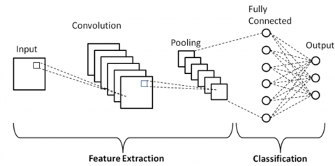
CNN is a deep learning model proposed by Yann LeCun [15] that can classify digital images and train systems with large amounts of data. CNNs have three types of layers: convolutional layers, pooling layers, and fully connected layers [16, 17] as shown in Figure 1.
Figure 1. Architecture of CNN
The convolutional layer functions to apply a set of filters or kernels to the input image. These filters are used to detect various features in the image, such as edges, corners, and textures. This process produces feature maps that identify the location and intensity of specific features within the image. Each filter works by combining all the pixels in the input image, resulting in diverse feature maps [18].
The pooling layer, often implemented as max-pooling or average-pooling, aims to reduce the dimensions of the feature maps. This layer helps decrease the number of parameters and computations within the network while retaining important information from the feature maps generated by the convolutional layer. By reducing dimensions, the pooling layer also helps control overfitting, making the model more generalizable to new data [18].
The fully connected layer, or dense layer, is the final stage in CNNs where all neurons are connected to each other. This layer is responsible for classifying based on the features extracted and processed by the convolutional and pooling layers. Each neuron in the fully connected layer receives input from all neurons in the previous layers, allowing the network to learn complex feature combinations and make final decisions regarding image classification [18].
2.2 Architecture MobileNetV2
MobileNetV2 is an advanced model that builds on MobileNetV1, showing improved accuracy with fewer parameters compared to its predecessor. MobileNetV2 is a CNN architecture designed to address the need for high computational resources [19]. In the MobileNet architecture, the convolution process is divided into two parts: depthwise convolution and pointwise convolution. This differentiates MobileNetV2 from traditional CNN architectures where convolutional layers have filters of varying thickness, depending on the thickness of the input image. MobileNetV2 presents two new features: linear bottlenecks and shortcut connections between bottlenecks as shown in Table 1 [20, 21].
Table 1. Architecture of MobileNetV2
|
Input |
Operator |
t |
c |
n |
s |
|
2242 × 3 |
Conv2d |
- |
32 |
1 |
2 |
|
1122 × 32 |
Bottleneck |
1 |
16 |
1 |
1 |
|
1122 × 16 |
Bottleneck |
6 |
24 |
2 |
2 |
|
562 × 24 |
Bottleneck |
6 |
32 |
3 |
2 |
|
282 × 32 |
Bottleneck |
6 |
64 |
4 |
2 |
|
142 × 64 |
Bottleneck |
6 |
96 |
3 |
1 |
|
142 × 96 |
Bottleneck |
6 |
160 |
3 |
2 |
|
72 × 160 |
Bottleneck |
6 |
320 |
1 |
1 |
|
72 × 320 |
Conv2d 1 × 1 |
- |
1280 |
1 |
1 |
|
72 × 1280 |
Avgpool 7 × 7 |
- |
- |
1 |
- |
|
1 × 1 × 1280 |
Conv2d 1 × 1 |
- |
k |
- |
- |
Linear bottlenecks help preserve important information through network layers by reducing information loss during compression and decompression processes. Meanwhile, shortcut connections, similar to residual connections in ResNet, allow for better information flow between layers, speeding up convergence and improving model performance [20].
2.3 Confusion matrix
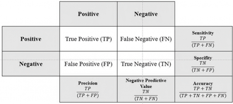
A confusion matrix is a tool used to evaluate the performance of a classification model in detecting diseases on corn leaves. This matrix shows the model's predicted results compared to the actual data as shown in Figure 2 [22, 23], It includes True Positive (TP) for correctly predicted diseases, True Negative (TN) for correctly predicted absence of disease, False Positive (FP) for incorrectly predicted diseases, and False Negative (FN) for incorrectly predicted absence of disease. By using a confusion matrix, metrics such as accuracy, precision, recall, specificity, and F1 score can be calculated, which helps in assessing the model's effectiveness and identifying and correcting prediction errors to improve disease detection performance [24, 25].
Figure 2. Confusion matrix
3.1 Dataset
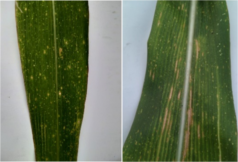
This study uses dataset consists of 4,000 images of corn leaf that has diseases. The corn leaf dataset was taken from corn farmers in the Sampang area of Madura Island, Indonesia. These images are divided into four classes: ['Leaf Spot', 'Healthy Leaf', 'Leaf Blight', 'Leaf Rust'] as depicted in Figure 3.
(a) Leaf Spot (b) Leaf Blight
(c) Healthy (d) Leaf Rust
Figure 3. The corn leaf disease
3.2 Analysis
Figure 4 illustrates the system flow that has been designed and implemented. Below is an explanation covering each stage of the system, from input to output, as well as the processes occurring between the components.
Figure 4. Diagram of the system
Dataset of this research must be well prepared to provide appropriate research object. There are four classes that divide images of corn leaf diseases from dataset of this study: ['Leaf Spot', 'Healthy Leaf', 'Leaf Blight', 'Leaf Rust']. Dataset consist of 4,000 images divided into 1,000 images for each class.
Resizing the image in dataset is the preprocessing used in this study. This step is utilized to standardize the image size by reducing it resolution from 3000 × 4000 pixels to 224 × 224 pixels. Additionally, resizing helps to simplify the computation process [22].
After the images are resized, the dataset is split into two parts using the K-Fold cross-validation method, with 80% for training and 20% for testing. This ensures that the model can learn from the majority of the available data and is tested with data that was not used during training to objectively measure its performance.
At this stage, the model is trained using the training data. During the training process, the model is also validated using a subset of the training data to monitor and prevent overfitting. This validation helps in adjusting the model's hyperparameters for optimal performance.
The two main optimizers used are Adam and RMSProp. These optimizers are responsible for managing weight updates in the neural network during training. Adam (Adaptive Moment Estimation) and RMSProp (Root Mean Square Propagation) were chosen to evaluate which optimizer performs better in handling convergence issues and accelerating the training process with adaptive learning rate adjustments.
This study also implements a classification model built using the MobileNetV2 architecture and employs parameters such as learning rate, dense layers, batch size, and optimizers Adam and RMSProp.
The final step is model evaluation. The trained and tested model is assessed to measure its overall performance. This evaluation includes measuring metrics such as accuracy, precision, recall, and F1 score.
This section explains about the results of the experiments on classification of corn leaf disease using the MobileNetV2 model. The data is partitioned into 80% and 20% of training and testing. Adaptive moment estimation (Adam) and root means square propagation (RMSProp) were used as the optimizers in these experiments with learning rates of 0.0001 and 0.05, respectively. Furthermore, the experiments exploited batch sizes of 64 and 32. The results of the experiments from scenario 1 to scenario 8 are described in Table 2.
Table 2 shows the results of the experiment with 8 different scenarios with different optimizers and batch sizes. The RMSprop optimizer has an accuracy of 99.34% better than using the Adam optimizer of 98.87% in the case of corn leaf disease classification. While Batch Size can affect the accuracy of around 1%.
Table 2. Test result
|
Trials |
Learning Rate |
Batch |
Optimizer |
High Accuracy |
|
Scenario 1 |
0.05 |
64 |
Rmsprop |
88.63% |
|
Scenario 2 |
0.05 |
32 |
Rmsprop |
87.15% |
|
Scenario 3 |
0.05 |
64 |
Adam |
86.64% |
|
Scenario 4 |
0.05 |
32 |
Adam |
85.04% |
|
Scenario 5 |
0.0001 |
64 |
Rmsprop |
99.34% |
|
Scenario 6 |
0.0001 |
32 |
Adam |
98.28% |
|
Scenario 7 |
0.0001 |
32 |
Rmsprop |
98.01% |
|
Scenario 8 |
0.0001 |
64 |
Adam |
98.87% |
Figure 5 explained that based on the testing results of the MobileNetV2 model with a learning rate of 0.05, batch size of 64, and RMSProp optimizer, there is a significant variation in model performance across several epochs. Training accuracy shows a consistent improvement, starting from 47.30% in the first epoch and reaching 88.63% in the final epoch. Training precision also follows a similar trend, with a minimum value of 45.30% and a maximum of 88.64%. Training recall ranges from 47.30% to 88.63%, and the training F1 score varies between 45.36% and 88.64%. For validation, validation accuracy starts at a low value of 25.00% and increases to 84.69% by the final epoch. Validation precision fluctuates, with a minimum of 36.53% and a maximum of 84.87%. Validation recalls ranges from 25.00% to 84.69%, while the validation F1 score varies from 65.33% to 84.75%. Training loss shows a decrease from 1.2339 at the beginning of testing to 0.3179 in the final epoch, indicating that the model is learning to reduce errors over time. Conversely, validation loss starts at 1.5084 and decreases to 0.4133, reflecting the model's improving ability to generalize to new data as the epochs progress. Overall, this graph shows that the model experiences significant improvement in performance metrics such as accuracy, precision, recall, and F1 score for both training and validation over time, while the training and validation loss decreases. This indicates an enhancement in the model's ability to make predictions more accurately and efficiently.
Figure 5. Graphic results of scenario 1 using RMSProp optimizer
Based on the testing results of the MobileNetV2 model with a learning rate of 0.05, batch size of 32, and RMSProp optimizer, there is significant variation in model performance across several epochs as shown in Figure 6. Training accuracy shows a consistent improvement, starting from 46.05% in the first epoch and reaching 87.15% in the final epoch. Training precision also improves, with a minimum of 44.98% and a maximum of 87.08%. Training recall ranges from 46.05% to 87.15%, and the training F1 score varies between 43.69% and 87.10%. For validation, validation accuracy starts at a low value of 25.31% and increases to 84.22% by the final epoch. Validation precision fluctuates, with a minimum of 58.20% and a maximum of 84.41%. Validation recalls ranges from 25.31% to 84.22%, while the validation F1 score varies from 57.43% to 84.21%. Training loss decreases from 1.2394 at the beginning of testing to 0.3436 in the final epoch, indicating that the model is learning to reduce errors over time.
Figure 6. Graphic results of scenario 2 using RMSProp optimizer
Conversely, validation loss starts at 1.4620 and decreases to 0.3824, reflecting the model's improving ability to generalize to new data as the epochs progress. Overall, this graph shows that the model experiences significant improvement in performance metrics such as accuracy, precision, recall, and F1 score for both training and validation over time, while the training and validation loss decreases. This indicates an enhancement in the model's ability to make predictions more accurately and efficiently.
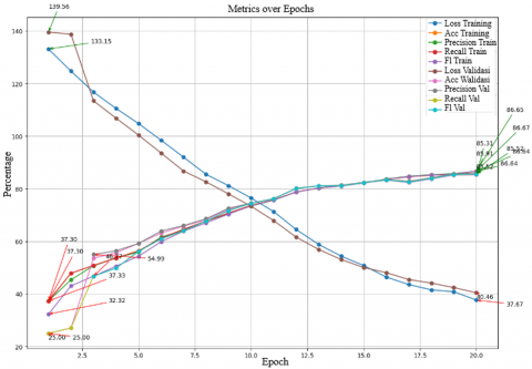
Based on Figure 7, it shows the results of testing the MobileNetV2 model with a learning rate of 0.05, batch size 64, and Adam optimizer, there is significant variation in model performance across several epochs. Training accuracy shows consistent improvement, starting from 37.30% in the first epoch and reaching 86.64% in the final epoch. Training precision also improves, with a minimum of 37.32% and a maximum of 86.67%. Training recall ranges from 37.30% to 86.64%, and the training F1 score varies between 32.32% and 86.65%. For validation, validation accuracy starts at a low value of 25.00% and increases to 85.31% by the final epoch. Validation precision fluctuates, with a minimum of 54.99% and a maximum of 85.91%. Validation recalls ranges from 25.00% to 85.31%, while the validation F1 score varies from 46.77% to 85.52%. Training loss decreases from 1.3315 at the beginning of testing to 0.3767 in the final epoch, indicating that the model is learning to reduce errors over time.
Figure 7. Graphic results of scenario 3 using Adam optimizer
Conversely, validation loss starts at 1.3956 and decreases to 0.4046, reflecting the model's improving ability to generalize to new data as the epochs progress. Overall, this graph shows that the model experiences significant improvement in performance metrics such as accuracy, precision, recall, and F1 score for both training and validation over time, while training and validation loss decreases, indicating an enhancement in the model's ability to make predictions more accurately and efficiently.
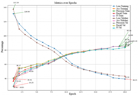
Figure 8 shows the testing results of the MobileNetV2 model with a learning rate of 0.05, batch size of 32, and Adam optimizer, there is significant variation in model performance across several epochs. Training accuracy shows consistent improvement, starting from 36.17% in the first epoch and reaching 85.04% in the final epoch. Training precision also improves, with a minimum of 40.85% and a maximum of 84.98%. Training recall ranges from 36.17% to 85.04%, and the training F1 score varies between 29.25% and 85.01%. For validation, validation accuracy starts at a low value of 28.91% and increases to 83.28% by the final epoch. Validation precision fluctuates, with a minimum of 39.46% and a maximum of 83.53%. Validation recalls ranges from 28.91% to 83.28%, while the validation F1 score varies from 49.85% to 83.35%. Training loss decreases from 1.3099 at the beginning of testing to 0.3925 in the final epoch, indicating that the model is learning to reduce errors over time. Conversely, validation loss starts at 1.3729 and decreases to 0.4334, reflecting the model's improving ability to generalize to new data as the epochs progress. Overall, this graph shows that the model experiences significant improvement in performance metrics such as accuracy, precision, recall, and F1 score for both training and validation over time, while training and validation loss decreases, indicating an enhancement in the model's ability to make predictions more accurately and efficiently.
Figure 8. Graphic results of scenario 4 using Adam optimizer
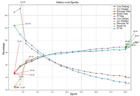
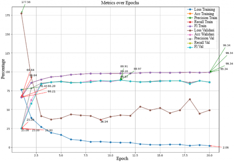
Figure 9 presents the experiment results of scenario 5 utilized the MobileNetV2 model with a learning rate of 0.0001, batch size of 64, and RMSProp optimizer. There is significant variation in model performance through several epochs. Training accuracy demonstrates consistent improvement, starting from 66.64% in the first epoch and reaching 99.34% in the final epoch. Training precision also presents similar advances, with a minimum of 66.20% and a maximum of 99.34%. The minimum result of training recall was 66.64% and the maximum reaches 99.34%. The training F1 score had lowest value of 66.21% and highest value of 99.34%. For validation, validation accuracy starts at a low value of 25.00% and increases to 88.91% by the final epoch. Validation precision fluctuates, with a minimum of 78.24% and a maximum of 89.20%. Validation recalls ranges from 25.00% to 88.91%, while the validation F1 score varies from 57.86% to 88.97%. Training loss decreases from 0.7640 at the beginning of testing to 0.0206 in the final epoch, indicating that the model is learning to reduce errors over time. Conversely, validation loss starts at 1.7756 and decreases to 0.3654, reflecting the model's improving ability to generalize to new data as the epochs progress. Overall, this graph shows that the model experiences significant improvement in performance metrics such as accuracy, precision, recall, and F1 score for both training and validation over time, while training and validation loss decreases, indicating an enhancement in the model's ability to make predictions more accurately and efficiently.
Figure 9. Graphic results of scenario 5 using RMSProp optimizer
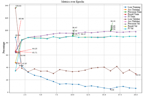
Figure 10 shows the testing results of the MobileNetV2 model with a learning rate of 0.0001, batch size of 32, and Adam optimizer, there is significant variation in model performance across several epochs. Training accuracy shows consistent improvement, starting from 65.90% in the first epoch and reaching 98.28% in the final epoch. Training precision also improves similarly, with a minimum of 65.71% and a maximum of 98.29%. Training recall ranges from 65.90% to 98.28%, and the training F1 score varies between 64.25% and 98.28%. For validation, validation accuracy starts at a low value of 47.97% and increases to 90.47% by the final epoch. Validation precision fluctuates, with a minimum of 65.54% and a maximum of 90.44%. Validation recall ranges from 47.97% to 90.47%, while the validation F1 score varies from 34.40% to 90.34%. Training loss decreases from 0.8849 at the beginning of testing to 0.0538 in the final epoch, indicating that the model is learning to reduce errors over time. Conversely, validation loss starts at 1.3602 and decreases to 0.2959, reflecting the model's improving ability to generalize to new data as the epochs progress. Overall, this graph shows that the model experiences significant improvement in performance metrics such as accuracy, precision, recall, and F1 score for both training and validation over time, while training and validation loss decreases, indicating an enhancement in the model's ability to make predictions more accurately and efficiently.
Figure 10. Graphic results of scenario 6 using Adam optimizer
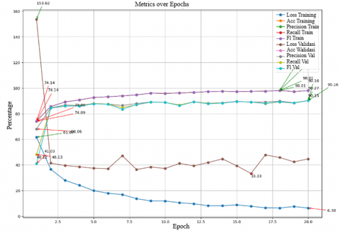
Figure 11 shows the testing results of the MobileNetV2 model with a learning rate of 0.0001, batch size of 32, and RMSProp optimizer, there is significant variation in model performance across several epochs. Training accuracy shows consistent improvement, starting from 74.14% in the first epoch and reaching 98.01% in the final epoch. Training precision also improves similarly, with a minimum of 74.06% and a maximum of 98.01%. Training recall ranges from 74.14% to 98.01%, and the training F1 score varies between 74.09% and 98.01%. For validation, validation accuracy starts at a low value of 48.13% and increases to 90.16% by the final epoch. Validation precision fluctuates, with a minimum of 68.06% and a maximum of 90.27%. Validation recall ranges from 48.13% to 90.16%, while the validation F1 score varies from 41.03% to 90.15%. Training loss decreases from 0.6167 at the beginning of testing to 0.0638 in the final epoch, indicating that the model is learning to reduce errors over time. Conversely, validation loss starts at 1.5362 and decreases to 0.3333, reflecting the model's improving ability to generalize to new data as the epochs progress. Overall, this graph shows that the model experiences significant improvement in performance metrics such as accuracy, precision, recall, and F1 score for both training and validation over time, while training and validation loss decreases, indicating an enhancement in the model's ability to make predictions more accurately and efficiently.
Figure 11. Graphic results of scenario 7 using RMSProp optimizer
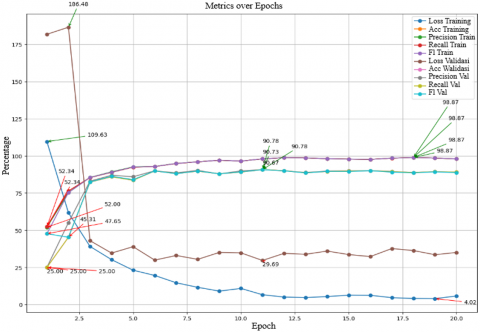
Figure 12 shows the testing results of the MobileNetV2 model with a learning rate of 0.0001, batch size of 64, and Adam optimizer, there is significant variation in model performance across several epochs. Training accuracy shows consistent improvement, starting from 52.34% in the first epoch and reaching 98.87% in the final epoch. Training precision also improves similarly, with a minimum of 51.99% and a maximum of 98.87%. Training recall ranges from 52.34% to 98.87%, and the training F1 score varies between 47.65% and 98.87%. For validation, validation accuracy starts at a low value of 25.00% and increases to 90.78% by the final epoch. Validation precision fluctuates, with a minimum of 55.16% and a maximum of 90.73%. Validation recalls ranges from 25.00% to 90.78%, while the validation F1 score varies from 82.44% to 90.67%. Training loss decreases from 1.0963 at the beginning of testing to 0.0402 in the final epoch, indicating that the model is learning to reduce errors over time. Conversely, validation loss starts at 1.8648 and decreases to 0.2969, reflecting the model's improving ability to generalize to new data as the epochs progress. Overall, this graph shows that the model experiences significant improvement in performance metrics such as accuracy, precision, recall, and F1 score for both training and validation over time, while training and validation loss decreases, indicating an enhancement in the model's ability to make predictions more accurately and efficiently.
Figure 12. Graphic results of scenario 8 using Adam optimizer
Table 3 shows the best test results, namely in scenario 5 with a learning rate of 0.0001 with a batch size of 64 and using the RMSProp optimizer with accuracy, precision and recall and F1 score of 99.34%.
Table 3. Best test result
|
Trials |
Accuracy (%) |
Precision (%) |
Recall (%) |
F1 Score (%) |
|
Scenario 1 |
88.63 |
88.64 |
88.63 |
88.64 |
|
Scenario 2 |
87.15 |
87.08 |
87.15 |
87.10 |
|
Scenario 3 |
86.64 |
86.67 |
86.64 |
86.65 |
|
Scenario 4 |
85.04 |
84.98 |
85.04 |
85.01 |
|
Scenario 5 |
99.34 |
99.34 |
99.34 |
99.34 |
|
Scenario 6 |
98.28 |
98.29 |
98.28 |
98.28 |
|
Scenario 7 |
98.01 |
98.01 |
98.01 |
98.01 |
|
Scenario 8 |
98.87 |
98.87 |
98.87 |
98.87 |
The conclusion of this study indicates that corn is an important staple crop with high productivity and various benefits, including as livestock feed and industrial raw material. To address challenges in corn production, particularly related to diseases such as leaf rust and leaf blight, artificial intelligence-based detection technologies like Convolutional Neural Networks (CNNs) have been employed to identify diseases more efficiently. Based on the testing results of the MobileNetV2 model with a learning rate of 0.0001, batch size of 64, and RMSProp optimizer, there is significant variation in model performance across several epochs. Training accuracy shows consistent improvement, starting from 66.64% in the first epoch and reaching 99.34% in the final epoch. Training precision also improves similarly, with a minimum of 66.20% and a maximum of 99.34%. Training recall ranges from 66.64% to 99.34%, and the training F1 score varies between 66.21% and 99.34%. For validation, validation accuracy starts at a low value of 25.00% and increases to 88.91% by the final epoch. Validation precision fluctuates, with a minimum of 78.24% and a maximum of 89.20%. Validation recalls ranges from 25.00% to 88.91%, while the validation F1 score varies from 57.86% to 88.97%. Training loss decreases from 0.7640 at the beginning of testing to 0.0206 in the final epoch, indicating that the model is learning to reduce errors over time. Conversely, validation loss starts at 1.7756 and decreases to 0.3654, reflecting the model's improving ability to generalize to new data as the epochs progress. Overall, the CNN model based on MobileNetV2 proves effective in classifying diseases in corn leaves, and the results can be used to develop an automated detection system that will assist farmers and researchers in managing and improving corn production more efficiently.
We convey our appreciation to Kemenristek DIKTI for the data environment that is provided up until the conclusion of this study. We also express our gratitude to the Faculty of Engineering, University of Trunojoyo Madura, which has already given the researcher permission to conduct this study in the Multimedia Laboratory. In addition, we would like to express our gratitude to the researchers at the Multimedia Laboratory who have helped us to complete this study. This study supports the findings of DIKTI and LPPM at Universitas Trunojoyo Madura in accordance with number 101/E5/PG.02.00.PL/2024 and contract number 041/UN46.4.1/PT.01.03/2024.
[1] Lopez-Zuniga, L.O., Wolters, P., Davis, S., Weldekidan, T., Kolkman, J.M., Nelson, R., Hooda, K.S., Rucker, E., Thomason, W., Wisser, R., Balint-Kurti, P. (2019). Using maize chromosome segment substitution line populations for the identification of loci associated with multiple disease resistance. G3 Genes|Genomes|Genetics, 9(1): 189-201. https://doi.org/10.1534/g3.118.200866
[2] Hidayat, K., Nasikin, M.K., Rakhmawati. (2021). Product development of corn rice using value engineering method. IOP Conference Series: Earth and Environmental Science, 733: 1-8. https://doi.org/10.1088/1755-1315/733/1/012039
[3] Zhang, X., Qiao, Y., Meng, F., Fan, C., Zhang, M. (2018). Identification of maize leaf diseases using improved deep convolutional neural networks. IEEE Access, 6: 30370-30377. https://doi.org/10.1109/ACCESS.2018.2844405
[4] Sayyid, M.F.N. (2024). Klasifikasi penyakit daun jagung menggunakan metode cnn dengan image processing HE Dan CLAHE. Jurnal Teknik Informatika dan Teknologi Informasi, 4(1): 86-95. https://doi.org/10.55606/jutiti.v4i1.3425
[5] Putro, S.S., Syakur, M.A., Rochman, E.M.S., Rachmad, A. (2022). Comparison of backpropagation and ERNN methods in predicting corn production. Communications in Mathematical Biology and Neuroscience, 2022(10): 1-17. https://doi.org/10.28919/cmbn/7082
[6] Bantacut, T., Firdaus, Y.R., Akbar, M.T. (2015). Pengembangan jagung untuk ketahanan pangan, industri dan ekonomi corn development for food security, industry and economy. Jurnal Pangan, 24(2): 135-148. https://doi.org/10.33964/jp.v24i2.29
[7] LeCun, Y., Bengio, Y., Hinton, G. (2015). Deep learning. Nature, 521(7553): 436-444. https://doi.org/10.1038/nature14539
[8] Rachmad, A., Syarief, M., Rifka, S., Sonata, F., Setiawan, W., Rochman, E.M.S. (2022). Corn leaf disease classification using local binary patterns (LBP) feature extraction. Journal of Physics: Conference Series. IOP Publishing, 2406(1): 012020. https://doi.org/10.1088/1742-6596/2406/1/012020
[9] Rachmad, A., Fuad, M., Rochman, E.M.S. (2023). Convolutional neural network-based classification model of corn leaf disease. Mathematical Modelling of Engineering Problems, 10(2): 530-536. https://doi.org/10.18280/mmep.100220
[10] Mumpuni, A.N., Kholifah, A.N., Syahfitri, A.A., Febrian, F.W., Aulia, I.D., Priyanti, K.R. (2021). Organisme pengganggu yang menyerang benih tanaman jagung (Zea mays L.) dan pengendaliannya, Prosiding Seminar Nasional Biologi, 1(2): 1208-1216.
[11] Sartori, M., Nesci, A., Formento, Á., Etcheverry, M. (2015). Selection of potential biological control of Exserohilum turcicum with epiphytic microorganisms from maize. Revista Argentina de Microbiologia, 47(1): 62-71. https://doi.org/10.1016/j.ram.2015.01.002
[12] Kumar, Y., Koul, A., Singla, R., Ijaz, M.F. (2023). Artificial intelligence in disease diagnosis: A systematic literature review, synthesizing framework and future research agenda. Journal of Ambient Intelligence and Humanized Computing, 14(7): 8459-8486. https://doi.org/10.1007/s12652-021-03612-z
[13] Zhou, L., Yu, W. (2022). Improved convolutional neural image recognition algorithm based on LeNet-5. Journal of Computer Networks and Communications, 2022(1): 1636203. https://doi.org/10.1155/2022/1636203
[14] Anton, A., Nissa, N.F., Janiati, A., Cahya, N., Astuti, P. (2021). Application of deep learning using convolutional neural network (CNN) method for Women’ s skin classification. Scientific Journal of Informatics, 8(1): 144-153. https://doi.org/10.15294/sji.v8i1.26888
[15] LeCun, Y., Bengio, Y., Hinton, G. (2015). Deep learning. Nature, 521(7553): 436-444. https://doi.org/10.1038/nature14539
[16] Hassanpour, M., Malek, H. (2020). Learning document image features with SqueezeNet convolutional neural network. International Journal of Engineering, 33(7): 1201-1207. https://doi.org/10.5829/ije.2020.33.07a.05
[17] He, K., Zhang, X., Ren, S., Sun, J. (2016). Deep residual learning for image recognition. In Proceedings of the IEEE Conference on Computer Vision and Pattern Recognition, Las Vegas, NV, USA, pp. 770-778. https://doi.org/10.1109/CVPR.2016.90
[18] Andika, L.A., Pratiwi, H., Handajani, S.S. (2019). Klasifikasi penyakit pneumonia menggunakan metode convolutional neural network dengan optimasi adaptive momentum. Indonesian Journal of Statistics and Its Applications, 3(3): 331-340. https://doi.org/10.29244/ijsa.v3i3.560
[19] Zaelani F., Miftahuddin, Y. (2022). Perbandingan metode EfficientNetB3 dan MobileNetV2 untuk identifikasi jenis buah-buahan menggunakan fitur daun. Jurnal Ilmiah Teknologi Infomasi Terapan, 9(1): 1-11. https://doi.org/10.33197/jitter.vol9.iss1.2022.911
[20] Sandler, M., Howard, A., Zhu, M., Zhmoginov, A., Chen, L.C. (2018). Mobilenetv2: Inverted residuals and linear bottlenecks. In Proceedings of the IEEE Conference on Computer Vision and Pattern Recognition, Salt Lake City, UT, USA, pp. 4510-4520. https://doi.org/10.1109/CVPR.2018.00474
[21] Elshennawy, N.M., Ibrahim, D.M. (2020). Deep-pneumonia framework using deep learning models based on chest X-ray images. Diagnostics, 10(9): 649. https://doi.org/10.3390/diagnostics10090649
[22] Tharwat, A. (2021). Classification assessment methods. Applied Computing and Informatics, 17(1): 168-192. https://doi.org/10.1016/j.aci.2018.08.003
[23] Chen, L., Li, S., Bai, Q., Yang, J., Jiang, S., Miao, Y. (2021). Review of image classification algorithms based on convolutional neural networks. Remote Sensing, 13(22): 4712. https://doi.org/10.3390/rs13224712
[24] Mehdiyev, N., Enke, D., Fettke, P., Loos, P. (2016). Evaluating forecasting methods by considering different accuracy measures. Procedia Computer Science, 95: 264-271. https://doi.org/10.1016/j.procs.2016.09.332
[25] Chen, R.C., Dewi, C., Huang, S.W., Caraka, R.E. (2020). Selecting critical features for data classification based on machine learning methods. Journal of Big Data, 7(1): 52. https://doi.org/10.1186/s40537-020-00327-4