Khairan Marzuki*![]() | Apriani
| Apriani![]() | Mudawil Qulub
| Mudawil Qulub![]()
© 2025 The authors. This article is published by IIETA and is licensed under the CC BY 4.0 license (http://creativecommons.org/licenses/by/4.0/).
OPEN ACCESS
The coffee industry continues to rely on subjective human visual assessments to determine the roasting levels of coffee beans, which are prone to inconsistencies due to factors such as fatigue and lighting conditions. This study proposes an objective approach utilizing convolutional neural networks (CNNs) to classify coffee roasting levels (dark roast, medium roast, light roast, and unroasted). The dataset comprises 1,600 coffee bean images, divided into training and testing sets with ratios of 75:25. The model was developed using the LeNet architecture and optimized with Adaptive Gradient (Adagrad) and Adaptive Moment Estimation (Adam) algorithms. Experimental results demonstrated that Adam achieved a validation accuracy of 96.75% and a training accuracy of 99.06%, outperforming Adagrad, which achieved a validation accuracy of 48.25% and a training accuracy of 51.59% at the 25th iteration. These findings confirm Adam's superiority in producing an optimal model. The proposed system effectively classifies coffee bean roasting levels with high precision, providing a reliable alternative to human-based evaluation. Future studies may focus on testing the model with larger datasets to further evaluate its scalability and robustness.
coffee bean, coffee roaster, convolutional neural network, image classification, optimization algorithm, LeNet architecture
Coffee beans are one of the most widely traded agricultural commodities in the world [1, 2]. Moreover, coffee beans represent a commodity with significant economic value [3]. Coffee is also one of the commodities that holds significant appeal for industry players today. The roasting of coffee beans is a critical stage in the coffee processing chain that can influence the quality of the coffee's taste and aroma [4]. The roasting process requires precise control of temperature and time, as these factors directly affect the sensory attributes of coffee, including aroma and flavor profile [5, 6]. The ideal ripeness level of coffee beans will yield optimal flavor [7]; however, this process often necessitates extensive expertise and experience. Errors in determining ripeness can lead to inconsistent outcomes, potentially diminishing product quality and consumer satisfaction.
In addition, a primary challenge currently faced in the coffee industry is the reliance on human visual assessment to determine the ripeness of coffee beans [8]. This assessment is subjective and may be affected by numerous factors, including weariness, lighting conditions, and personal experience [9]. Consequently, the determination of coffee bean ripeness is often inaccurate and inconsistent.
To address these issues, a more objective, efficient, and consistent solution is required. One promising method is the implementation of an intelligent system based on CNN, which has proven effective in handling visual data. CNN is derived from artificial neural network (ANN) algorithms, which are deep learning that mimic the neural networks in the brain to classify images. CNN can autonomously learn features from complex images, accept input in the form of pictures, identify objects or aspects present within a given image, and distinguish between different images [10].
This research aims to develop a model for classifying the maturity of coffee beans using CNN with a LeNet architecture, which is known for its simplicity yet capable of yielding good results in image classification tasks. The maturity levels of roasted coffee are categorized into four levels: dark roasted, medium roasted, light roasted, and unroasted. The optimal maturity level for coffee is found in the light, medium, and dark roasted stages [11].
A variety of research related to coffee beans, such as that conducted by Susanti et al. [12], investigates the implementation of an electronic nose (e-nose) and ANN to differentiate between Arabica, Robusta, and non-bean coffee powders. The results indicate that the TGS 2602 and TGS 2611 sensors demonstrated significant sensitivity in distinguishing the types of coffee. By incorporating the ANN method, the developed system achieved an accuracy of 91.90%. The identified gap in the study lies in its presentation of a different perspective on classifying coffee bean types. The classification of coffee bean types is conducted based on data from an E-Nose, visualized using LabView software, and followed by a learning process using ANN to develop a model capable of distinguishing coffee types. In contrast, our study focuses on classifying the roasting levels of coffee beans after the roasting process, without considering the coffee bean types. Furthermore, the machine learning method employed in our study is an advancement of ANN, namely CNN.
Research by Alamri et al. [13], examined the classification of Arabica coffee into three categories: light, medium, and dark, using simulated data based on characteristics such as color, chemical composition, and antioxidant laboratory tests. The methods employed include support vector machine (SVM), K-Nearest Neighbors (KNN), Random Forest, Naive Bayes, and the decision tree algorithm C4.5. The results indicate that coffee types can be accurately classified by utilizing information on color, chemical composition, and antioxidant content. The identified gap is that the study shares similarities in classifying the roasting levels of coffee beans; however, there is a difference in the methods used for classification. The study developed classification models using SVM, KNN, Random Forest, Naive Bayes, and the decision tree algorithm C4.5. In contrast, our research focuses on developing a classification model using CNN.
Research by Anto et al. [14], utilized the LAB Color model and CNN to identify the roasting maturity level of coffee. The LAB Color model analyzed color using three components: lightness (L), the green-to-red axis (A), and the blue-to-yellow axis (B), providing more accurate results compared to the RGB model. The CNN was employed to classify the roasting levels, achieving a training accuracy of 99.552% at the 14th iteration and the best validation accuracy of 91.8% at the 10th iteration. The combination of these models proved effective for analyzing coffee roasting maturity levels. The identified gap in the study lies in its similarity in classifying coffee bean roasting levels using CNN. However, the primary difference is in the CNN architecture employed. Our study utilizes the LeNet architecture, while the previous study adopts the HyperResNet architecture. Furthermore, the previous study does not specify the type of CNN optimization applied.
Research by Vilcamiza et al. [15], utilized a CNN model to classify coffee bean images based on roasting maturity levels. The optimization model applied was Adam, implemented on the NVIDIA Jetson Nano module. The CNN model successfully identified various roasting levels, including correct roasting, false under-roasting, false-optimum roasting, and false over-roasting. The results indicate that the CNN model achieved a classification accuracy of 91.33%. The identified gap in the study lies in the differences in the type of classification performed. Furthermore, the study does not provide a detailed explanation of the CNN architecture used, and the CNN optimization applied is limited to the Adam algorithm.
Research by Auliya et al. [16], examines the implementation of convolutional neural networks (CNN) to classify green coffee beans into three categories: green, dark, and light. The dataset consists of 360 images. The results show that the 80:20 data split scenario achieved the best accuracy of 81.67% at the 30th epoch. The identified gap lies in the differences in the coffee bean objects being classified. The previous study focused on classifying green coffee beans into three categories: green, dark, and light. In contrast, our study focuses on classifying coffee beans after the roasting process. Furthermore, there are differences in the optimization methods applied to the CNN model.
Previous research has examined the use of CNNs in classifying the ripeness levels of coffee beans after roasting; however, only a few studies have developed CNN models utilizing the LeNet architecture with various optimizations. Therefore, the novelty of this research lies in developing the most optimal model using CNN with the LeNet architecture and a range of CNN optimizations to classify the ripeness levels of coffee beans post-roasting with high accuracy.
In this study, we implement CNN with a LeNet architecture that has been trained to classify the roasting maturity levels of coffee beans. The dataset utilized encompasses a variety of images depicting roasted coffee beans, enabling the model to learn from the existing visual variations. The main goal of this classification is to produce a precise evaluation of the maturity degree of the coffee beans. This project aims to identify the most suitable LeNet-based CNN model for accurately assessing the maturity degree of coffee beans.
2.1 Dataset
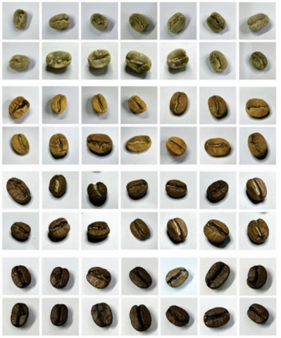
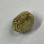
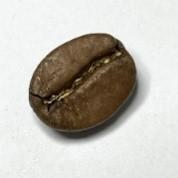
This dataset comprises image of coffee beans that have been roasted at various levels of maturity, including dark roast, medium roast, light roast, and unroasted coffee beans. Raw coffee beans were incorporated into the dataset to enhance data diversity. This study comprises a total of 1,600 photos, with each categorization consisting of 400 photographs. The image data is partitioned into two segments: a training dataset consisting of 1,200 images and a prediction dataset of 400 images. Each maturity level is subdivided into 300 photos for training and 100 images for prediction. The dimensions of the dataset photos are 224 pixels by 224 pixels. The dataset utilized in this research is depicted in Figure 1.
Figure 1. Dataset
2.2 CNNs
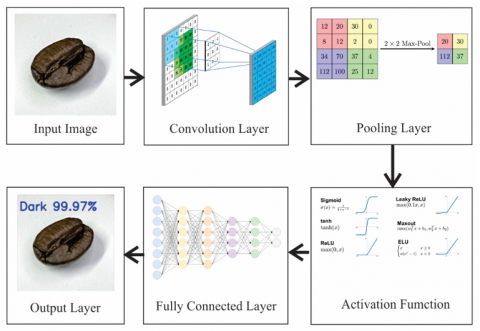
CNN is an avenue of ANN specifically engineered to analyze image data. The CNN method is highly effective for tasks such as image segmentation [17, 18], object detection [17, 19], image classification [20, 21], and others. One of the key advantages of CNN lies in its convolutional layers, which enable the network to automatically identify important features of an image through the processes of convolution and pooling [22, 23]. Figure 2 illustrates the components that make up CNN.
Figure 2. CNN building blocks
This study uses the CNN method to classify of roasting maturity levels of coffee beans [24]. In its usage, CNN comprises several core components, beginning with the input image serving as the initial data, the convolutional layer extracting features from the image, the pooling layer reducing the information to a simpler form, the activation function adding non-linearity to the network, the fully connected layer linking all previous neurons, and the output layer providing the final prediction [25]. The classification is conducted through the following steps:
2.2.1 Input image
The input image in CNN is data used for object classification by extracting features from the image [26]. In this study, the CNN input consists of images of roasted coffee beans. These images are categorized into four types: dark roast, medium roast, light roast, and unroasted coffee beans. The image size used is 224×224 pixels, with Red Green Blue (RGB) color channels, resulting in an input shape of 224×224×3 pixels.
2.2.2 Convolutional layer
The convolutional layer is a core component in constructing a CNN, specifically used for processing data in the form of images or audio. The convolutional layer performs a convolution operation on the input image to extract critical information, including texture, color, edges, and roasting patterns of coffee beans.
The input to the CNN is in the form of an RGB image, which means the CNN input is a three-dimensional matrix composed of height, width, and depth. The height and width components of the matrix can be represented as pixel data, while the depth component is represented by color channels. The operation of the convolutional layer involves the application of filters (kernels) to perform convolution on the input data. Convolution is performed by sliding a filter across the image data [27]. The filter used is smaller than the input image dimensions, allowing it to detect specific features. A commonly used filter size is a 3×3 matrix, which provides a balance between computational efficiency and feature detection accuracy.
Whenever the filter traverses a segment of the input, the dot product of the filter's pixel elements and the input data pixels is computed, followed by summing. The result of this operation is a matrix called a feature map, activation map, or convolved feature. The filter then shifts progressively and repeats this process until the entire image area is covered [28, 29]. The convolution operation involving the filter (K) and the input image (x) is articulated in Eq. (1).
$S(i, j)=\sum_m \sum_n X(i+m, j+n) \times K(m, n)$ (1)
where S(i,j) specifies the feature map at coordinates (i,j), K(m,n) signifies the position of the filter (kernel), and X(i+m, j+n) indicates the position of the input picture.
2.2.3 Activation function
The activation function plays a crucial role in modeling the relationship between input data and output. It is used to perform nonlinear data transformations [30]. In CNNs, activation functions are typically divided into three categories: Rectified Linear Unit (ReLU), sigmoid, and softmax functions. The ReLU function is among the most often utilized activation functions in CNN. ReLU functions by transforming negative values to zero while preserving positive values. The ReLU function functions by eliminating all negative values produced during the convolution process, permitting only positive values to proceed to the subsequent layer. The mathematical representation of the ReLU function is illustrated in Eq. (2).
$f(x)=\max (0, x)$ (2)
The subsequent activation function is the sigmoid function. In the sigmoid function, the input values will be converted into values in the range of 0 to 1. This function is commonly employed in binary classification tasks. The equation for the sigmoid function is presented in Eq. (3).
$f(x)=\frac{1}{1+e^{-x}}$ (3)
The Softmax algorithm subsequently converts the output of the last layer into probabilistic values across several classes. This study uses the Softmax function to allocate probability values to each class, as the categorization encompasses many classes. The class with the highest likelihood is deemed the prediction generated by the CNN. The Softmax function is defined by Eq. (4).
$f(x)=\frac{2}{1+e^{-2 x}}-1$ (4)
2.2.4 Pooling layer
The pooling layer serves to diminish the dimensionality of features produced during the convolution process while retaining essential information from the data. In a CNN, the pooling layer combines a group of neurons in the feature map into a single value. The pooling technique is categorized into two types: average pooling and max pooling [27-29].
Max pooling functions to extract the maximum value from a small area, such as the maximum value from a 2×2 or 3×3 matrix within the feature map, which is then used as the representation for that area. In the max pooling process, only the dominant features are retained for the subsequent steps, while the other features are disregarded. The equation for max pooling can be shown in Eq. (5).
$S(i, j)=\max \left(X_{i: i+k-1, j: j+k-1}\right)$ (5)
2.2.5 Fully connected layer
In CNN, the fully connected (FC) layer is characterized by each neuron being directly linked to every neuron in the succeeding layer underneath it. The principal role of the FC layer is to integrate the features derived from the convolutional and pooling layers and to render judgments based on those features. At this layer, the spatial representation generated by the preceding layers is converted into a one-dimensional vector, which is subsequently transmitted to the fully connected layer for classification or regression [27-29].
In the FC layer, each neuron receives input from all the neurons in the preceding layer, and each input is associated with a corresponding weight. Each neuron performs a linear operation on the input, followed by applying an activation function (such as ReLU or sigmoid) to produce a non-linear output. This process can be viewed as a traditional neural network (fully connected neural network) integrated with the CNN architecture for the final decision-making stage.
For instance, suppose we have an input vector from the previous layer $x=\left[x_1, x_2, \ldots, x_n\right]$, the output of the j-th neuron in the FC layer is calculated using Eq. (5) as follows:
$y_j=f\left(\sum_{i=1}^n w_{i j} x_i+b_j\right)$ (6)
where, wij is a weight in the fully connected layer that connects neuron i from the previous layer to neuron j. xi is the input of neuron i in the previous layer. bj represents the bias associated with neuron j. f(.) is a function implemented after a linear operation such as ReLU, sigmoid, or Softmax (for classification).
2.2.6 Output layer
The output layer in a CNN function as the final layer that generates predictions based on the characteristics retrieved and processed by the preceding layers, including the layer of convolution, pooling layer, and fully connected layers [31]. The output layer's major job is to convert abstract representations of learnt features into interpretable outputs, usually as classes (for classification) or continuous values (for regression). The output layer of a classification job often employs the Softmax activation function to provide a probability distribution across multiple classes.
2.3 LeNet architecture
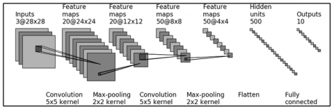
LeNet is one of the early architectures of CNN [32, 33]. In 1989, Yann LeCun and his team developed a CNN model trained using the backpropagation method to read handwritten text. This model was successful in identifying handwritten postal codes. The structure subsequently became the foundation of what is known as LeNet. In this study, the classification system employs the LeNet architecture, with the network structure illustrated in Figure 3.
Figure 3. LeNet architecture
In this study, the data utilized consists of coffee bean images in RGB color format, with dimensions of 28×28 pixels. The first stage involves a convolution process using a 5×5 kernel to generate a sequence of feature maps measuring 24×24, comprising 20 feature maps. Following this, max pooling is performed with a 2×2 kernel to reduce the size to 12×12 while maintaining the depth of 20 feature maps. In the second convolution, a 5×5 kernel is employed again to produce feature maps of size 8×8 with a depth of 50. This is followed by max pooling using a 2×2 kernel, which reduces the feature map size to 4×4, still retaining a depth of 50. The subsequent process is flattening, which converts the final feature map into a vector that is then input into the fully connected layer to generated the final predictions.
The results section describes the obtained findings gathered from your research. Provide appropriate figures and tables to effectively illustrate your results. Figures are used to present data trends or other visual information while tables are particularly useful when the exact values are important.
To determine the level of coffee roast maturity, this study develops a CNN algorithm based on the LeNet architecture to produce the most optimal model for classifying the maturity levels of coffee roasts. The maturity levels to be predicted are divided into three classifications: dark roast, medium roast, light rost, and green bean. These classifications represent general categories of coffee roast maturity; however, in practice, they can be challenging to distinguish visually due to their similar colors. The CNN algorithm is suitable for this task, as it is designed to analyze image data. The experiments conducted in this research aim to obtain an optimal model through training with various numbers of iterations. Additionally, several optimizers are employed in the applied CNN model to reduce the training iterations while achieving high accuracy. The optimizations utilized in this study are Adam and Adagrad. The testing was conducted to identify the most suitable optimization for the developed CNN model, aiming to achieve high accuracy while reducing the training and validation time. The training and validation data were divided with a ratio of 75:25.
3.1 Model training using adaptive gradient
Adaptive gradient (Adagrad) is an optimization algorithm employed for training models within CNN. The optimization concept utilized in the Adagrad algorithm is adaptive gradient descent. The Adagrad algorithm's adaptability entails assigning variable learning rates to each parameter, contingent upon the frequency of updates received during training. Thus, the Adagrad algorithm elevates the learning rate for seldom changed parameters while diminishing the learning rate for frequently updated values. This functionality enables enhanced optimization inside CNN designs.
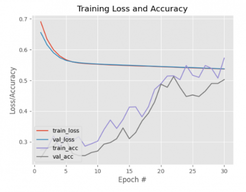
The experiments conducted in model training using Adagrad involved analyzing the training loss and accuracy generated during the learning process with variations in learning iterations in multiples of five, ranging from the 5th iteration to the 30th iteration. The outcomes of this experiment are depicted in Figure 4.
According to the test results presented in Table 1, the training accuracy improved from 27.98% to 43.09%. However, this improvement is not particularly significant. Conversely, a consistent decrease is observed in the training loss values. Nevertheless, the validation accuracy did not exhibit any meaningful change and remained at 34.5%, while the validation loss showed a decrease. From this data, it can be concluded that at the 5th and 10th iterations, despite the increase in training accuracy, the overall accuracy level remains relatively low. This indicates that the model produced is not yet optimal in performing classification.
Figure 4. Learning using Adagrad algorithm with epoch 30
Table 1. Training loss and accuracy test results using Adagard optimisation in CNN
|
Epoch |
Train Accuracy |
Train Loss |
Validation Accuracy |
Validation Loss |
|
5 |
0.2798 |
0.5811 |
0.345 |
0.5742 |
|
10 |
0.4309 |
0.5519 |
0.345 |
0.5537 |
|
15 |
0.37 |
0.5517 |
0.3825 |
0.5525 |
|
20 |
0.3562 |
0.5485 |
0.3225 |
0.5508 |
|
25 |
0.5159 |
0.5372 |
0.4825 |
0.5376 |
|
30 |
0.5725 |
0.5368 |
0.5025 |
0.5375 |
At the 15th and 20th iterations, a decline in training accuracy was observed compared to the previous iterations, with values of 37% at the 15th iteration and 35.62% at the 20th iteration, respectively. This decline suggests that the model is beginning to struggle to learn patterns from the training data. This decrease is also evident in the validation accuracy, where at the 20th iteration, a drop indicates that the model is not only having difficulty learning from the training data but is also unable to perform well on the validation data. Furthermore, both training loss and validation loss also showed a decrease in these two iterations. This decrease in loss indicates that the model is experiencing fewer errors in its predictions; however, the drop in accuracy suggests that a reduction in loss alone is insufficient to guarantee an overall improvement in performance.
In the 25th and 30th iterations, the results demonstrated an increase in accuracy. In the 25th iteration, the accuracy reached 51.59%, while in the 30th iteration, the accuracy further improved to 57.25%. Additionally, validation accuracy also experienced an increase compared to the previous iterations, achieving a peak accuracy of 50.25% in the 30th iteration. This indicates that the model used successfully improved its performance with the increasing number of iterations. However, a similar trend was not observed in training loss or validation loss, as there were no significant changes. Both training loss and validation loss remained relatively stable throughout these iterations, suggesting that the model has reached a saturation point in its learning.
It can be concluded that in the 30th iteration, the model optimized using the Adagrad method achieved a validation accuracy of 50.25% and a training accuracy of 57.25%. Although the 30th iteration yielded the highest accuracy compared to other iterations, this accuracy level remains relatively low. This indicates that the application of the Adagrad optimization method in the CNN model has not been able to produce optimal performance in the classification of coffee roasting maturity. The low validation accuracy also suggests that the model is experiencing underfitting, which necessitates further exploration of alternative optimization methods or adjustments to the CNN architecture, such as the number of layers or filters used.
3.2 Model training using Adaptive Moment Estimation
Adaptive Moment Estimation (Adam) is a widely used optimization algorithm in CNN. The Adam optimization algorithm can effectively address problems with numerous parameters and large datasets. Adam updates parameters by utilizing the first moment estimate (mean) and the second moment estimate (uncorrected variance) of the gradients. This algorithm is designed to adjust the learning rate adaptively for every parameter, depending on the gradient moments.
Figure 5. Learning using the Adam algorithm with 30 epochs
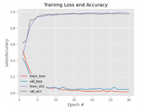
The experiments conducted in training the model using Adam involve analyzing the training loss and accuracy generated during the learning process with varying learning iterations in multiples of five, ranging from 5 to 30 iterations. The results of the conducted tests are illustrated in Figure 5.
The testing of the Adam optimization algorithm on the CNN was conducted to establish the best number of iterations for producing the most effective CNN model in classifying the roasting maturity levels of coffee beans. Based on the results from the tests conducted between the 5th and the 15th iterations, a significant increase in training accuracy was observed, rising from 95.29% at the 5th iteration to 98.03% at the 15th iteration. Additionally, validation accuracy also displayed a positive trend, increasing from 94.5% at the 5th iteration to 97% at the 15th iteration.
The enhancement in accuracy for both the training and validation datasets signifies that this model is becoming adept at discerning patterns within the data used for training, while also generalizing effectively to novel data. This suggests that the model not only succeeded in enhancing training accuracy but also maintained validation accuracy, thereby minimizing the risk of overfitting.
From the 20th to the 30th iteration, both training accuracy and prediction accuracy exhibited relatively high results. Training accuracy increased from 98.63% at the 20th iteration to 99.06% at the 25th iteration, which marked the point at which the highest training accuracy was achieved. However, by the 30th iteration, training accuracy experienced a slight decline to 98.8%. Meanwhile, prediction accuracy experienced minor fluctuations, starting at 97.25% at the 20th iteration, dipping slightly to 96.75% at the 25th iteration, and then rising again to 97.5% at the 30th iteration. Although there was a slight decline at the 25th iteration, this decrease was not significant and was followed by an increase in subsequent iterations.
Furthermore, the trends of training loss and validation loss generated by the CNN model using Adam optimization also demonstrated consistent decreases. The loss values remained consistently low and continued to decrease with additional iterations, signifying that the model was becoming progressively more adept at learning data patterns. The decrease in loss indicates a successful training procedure, as the model effectively reduced prediction errors throughout the learning phase.
From these testing results, it can be interpreted that although training accuracy continued to rise until the 25th iteration, the decline observed at the 30th iteration indicates potential overfitting at higher iterations. The performance of prediction accuracy, which exhibited minor fluctuations, may suggest that the model began to experience difficulties in generalizing to the test data in certain iterations, although its overall performance remained strong. Based on these results, the 25th iteration is identified as the most optimal for maintaining a balance between high training accuracy and stable prediction accuracy. The consistent decrease in both validation loss and training loss also signifies that this model is not only learning effectively but also demonstrating a trend toward reducing errors, which is crucial for ensuring good generalization capabilities across various iterations. The data and results are presented in greater detail in Table 2 and Figure 5 to illustrate the trends in accuracy and loss for each iteration.
Table 2. Results of the training loss and accuracy tests using Adam optimization in CNN
|
Epoch |
Train Accuracy |
Train Loss |
Validation Accuracy |
Validation Loss |
|
5 |
0.9529 |
0.1033 |
0.945 |
0.0954 |
|
10 |
0.9742 |
0.0431 |
0.97 |
0.0568 |
|
15 |
0.9803 |
0.0297 |
0.97 |
0.0496 |
|
20 |
0.9863 |
0.0224 |
0.9725 |
0.0485 |
|
25 |
0.9906 |
0.0141 |
0.9675 |
0.0718 |
|
30 |
0.988 |
0.0154 |
0.975 |
0.0443 |
3.3 Testing with various training-to-validation splits
After determining the appropriate optimization for the developed CNN model, further testing was conducted to analyze the performance of the CNN model under different data split scenarios. The training and validation data splits used in this study were 75:25, 80:20, and 90:10. The number of epochs used in the testing was 30. The Adam optimization algorithm was employed in this test because it produced better validation and training accuracy compared to Adagrad. Experimental results demonstrated that Adam achieved a validation accuracy of 96.75% and a training accuracy of 99.06%, outperforming Adagrad, which achieved a validation accuracy of 48.25% and a training accuracy of 51.59% at the 25th iteration. The testing results for the 75:25 data split are presented in Table 2, while the results for the 80:20 and 90:10 data splits are shown in Tables 3 and 4.
Table 3. Training-to-validation testing using the Adam optimization algorithm with an 80:20 data split scenario
|
Epoch |
Train Accuracy |
Train Loss |
Validation Accuracy |
Validation Loss |
|
5 |
0.9005 |
0.1748 |
0.9031 |
0.1578 |
|
10 |
0.9632 |
0.0656 |
0.9656 |
0.0582 |
|
15 |
0.9773 |
0.0443 |
0.9656 |
0.0405 |
|
20 |
0.9881 |
0.0232 |
0.9688 |
0.0390 |
|
25 |
0.9849 |
0.0260 |
0.9719 |
0.0318 |
|
30 |
0.9815 |
0.0214 |
0.9688 |
0.0356 |
Table 4. Training-to-validation testing using the Adam optimization algorithm with 90:10 data split scenario
|
Epoch |
Train Accuracy |
Train Loss |
Validation Accuracy |
Validation Loss |
|
5 |
0.9206 |
0.1586 |
0.9444 |
0.1435 |
|
10 |
0.9675 |
0.0555 |
0.9361 |
0.0957 |
|
15 |
0.9694 |
0.0443 |
0.9650 |
0.0563 |
|
20 |
0.9818 |
0.0275 |
0.9667 |
0.0479 |
|
25 |
0.9885 |
0.0192 |
0.9722 |
0.0391 |
|
30 |
0.9866 |
0.0245 |
0.9556 |
0.0729 |
Based on the testing results presented in Tables 2-4 with training-to-validation data split scenarios of 75:25, 80:20, and 90:10 using the Adam optimization algorithm, several important findings can be interpreted.
In the 75:25 data split scenario, the model achieved the highest validation accuracy of 97.50% at the 25th epoch, with a relatively low validation loss of 0.0443. In the 80:20 data split scenario, the highest validation accuracy of 97.19% was achieved at the 25th epoch, with the lowest validation loss recorded at 0.0318. The model demonstrated stable performance in this scenario, with training accuracy reaching 98.49% at the same epoch. Meanwhile, in the 90:10 data split scenario, the highest validation accuracy of 97.22% was achieved at the 25th epoch, with a validation loss of 0.0391. However, at the 30th epoch, the validation accuracy decreased to 95.56%, despite the training accuracy remaining high at 98.66%. This indicates that the model tends to overfit the training data when the validation dataset size is smaller.
Overall, the 80:20 data split scenario exhibited the most consistent performance, with more stable validation loss and high validation accuracy. Therefore, the recommended data split scenario is 80:20.
3.4 Classification results
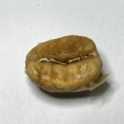
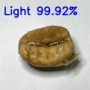
After developing the CNN model using the LeNet architecture and the Adagrad and Adam optimization algorithms, the model was applied to classify the ripeness levels of coffee beans following the roasting process. The experimental results suggest that the Adam optimization algorithm produced the most optimal model, with the best performance achieved at the 25th iteration. At this iteration, the model attained a validation accuracy of 96.75% and a training accuracy of 99.06%. The recommended training-to-validation data split scenario in this study is 80:20. This scenario has proven to deliver more stable validation performance, with a validation accuracy of 97.19%, a validation loss of 0.0318, and a training accuracy of 98.49% at the 25th iteration. This CNN model accepts static images as input, representing the varying ripeness of roasting maturity levels of coffee beans. The classification testing results for the ripeness of roasted coffee beans are presented in Table 5.
The findings of this study align with those reported in previous research [15, 16]. This study demonstrates that a CNN model with a LeNet architecture optimized using the Adam algorithm can effectively classify the roasting maturity levels of coffee beans after the roasting process. This research provides a significant contribution by complementing earlier studies that focused on the classification of roasting errors and the classification of raw coffee beans. Furthermore, these findings reinforce the potential of deep learning-based technologies to enhance efficiency and accuracy in the coffee industry, particularly in critical stages such as the classification of roasting maturity levels. Additionally, the results of this study pave the way for further developments, such as applying the approach to larger datasets or exploring other CNN architectures to improve model performance.
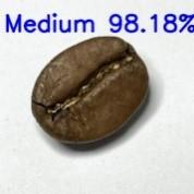
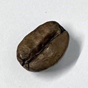
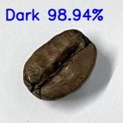
Table 5. The results of testing the classification of the maturity level of roasted coffee beans
|
Input |
Output |
Classification Result |
|
Green |
||
|
Light |
||
|
Medium |
||
|
Dark |
In this study, a CNN model has been successfully developed using the LeNet architecture along with two optimization algorithms, namely Adagrad and Adam. The Adam optimization demonstrated superior performance in generating the most optimal model. The experimental results demonstrated that Adam achieved a validation accuracy of 96.75% and a training accuracy of 99.06%, outperforming Adagrad, which achieved a validation accuracy of 48.25% and a training accuracy of 51.59% at the 25th iteration. These results indicate that the developed model has effectively classified the maturity level of post-roasted coffee beans with a very high accuracy rate. Furthermore, the successful application of Adam optimization suggests that this algorithm is more effective than Adagrad in accelerating the convergence process and achieving more accurate results, particularly with the dataset used in this classification.
The recommended training-to-validation data split scenario in this study is 80:20. This scenario has proven to deliver more stable validation performance, with a validation accuracy of 97.19%, a validation loss of 0.0318, and a training accuracy of 98.49% at the 25th iteration. The high performance of the model reflects the CNN's ability to recognize critical features related to the maturity levels of coffee beans, making it a reliable approach for applications in the coffee roasting industry. The findings of this study indicate that a CNN model with a LeNet architecture, optimized using the Adam algorithm, can effectively classify the roasting maturity levels of coffee beans after the roasting process. Future research may be conducted to evaluate the performance of this model on larger and more diverse datasets to enhance its generalization across various real-world conditions.
This study received funding from the Ministry of Education, Culture, Research, and Technology (Kemendikbudristek) through the fundamental research program. We express deep appreciation for the financial support received for this study and acknowledge all parties that contributed to the accomplishment of this research.
[1] Medina-Orjuela, M.E., Barrios-Rodríguez, Y.F., Carranza, C., Amorocho-Cruz, C., Gentile, P., Girón-Hernández, J. (2024). Enhancing analysis of neo-formed contaminants in two relevant food global commodities: Coffee and Cocoa. Heliyon, 10(10): e31506. https://doi.org/10.1016/j.heliyon.2024.e31506
[2] Chéron-Bessou, C., Acosta-Alba, I., Boissy, J., Payen, S., et al. (2024). Unravelling life cycle impacts of coffee: Why do results differ so much among studies? Sustainable Production and Consumption, 47: 251-266. https://doi.org/10.1016/j.spc.2024.04.005
[3] Fischer, E.F. (2021). Quality and inequality: Creating value worlds with third wave coffee. Socio-Economic Review, 19(1): 111-131. https://doi.org/10.1093/ser/mwz044
[4] Astuti, S.D., Wicaksono, I.R., Soelistiono, S., Permatasari, P.A.D., et al. (2024). Electronic nose coupled with artificial neural network for classifying of coffee roasting profile. Sensing and Bio-Sensing Research, 43: 100632. https://doi.org/10.1016/j.sbsr.2024.100632
[5] Di Palma, F., Iacono, F., Toffanin, C., Ziccardi, A., Magni, L. (2021). Scalable model for industrial coffee roasting chamber. Procedia Computer Science, 180: 122-131. https://doi.org/10.1016/j.procs.2021.01.362
[6] Rabelo, M.H.S., Borém, F.M., de Lima, R.R., de Carvalho Alves, A.P., et al. (2021). Impacts of quaker beans over sensory characteristics and volatile composition of specialty natural coffees. Food Chemistry, 342: 128304. https://doi.org/10.1016/j.foodchem.2020.128304
[7] Severin, H.G., Lindemann, B. (2024). Elasticity of coffee beans: A novel approach to understanding the roasting process. Journal of Food Engineering, 383: 112212. https://doi.org/10.1016/j.jfoodeng.2024.112212
[8] Alamsyah, A., Widiyanesti, S., Wulansari, P., Nurhazizah, E., et al. (2023). Blockchain traceability model in the coffee industry. Journal of Open Innovation: Technology, Market, and Complexity, 9(1): 100008. https://doi.org/10.1016/j.joitmc.2023.100008
[9] Tamayo-Monsalve, M.A., Mercado-Ruiz, E., Villa-Pulgarin, J.P., Bravo-Ortiz, M.A., et al. (2022). Coffee maturity classification using convolutional neural networks and transfer learning. IEEE Access, 10: 42971-42982. https://doi.org/10.1109/ACCESS.2022.3166515
[10] Paymode, A.S., Malode, V.B. (2022). Transfer learning for multi-crop leaf disease image classification using convolutional neural network VGG. Artificial Intelligence in Agriculture, 6: 23-33. https://doi.org/10.1016/j.aiia.2021.12.002
[11] Tsai, C.F., Jioe, I.P.J. (2021). The analysis of chlorogenic acid and caffeine content and its correlation with coffee bean color under different roasting degree and sources of coffee (Coffea Arabica Typica). Processes, 9(11): 2040. https://doi.org/10.3390/pr9112040
[12] Susanti, R., Zaini, Z., Hidayat, A., Alfitri, N., Rusydi, M.I. (2023). Identification of coffee types using an electronic nose with the backpropagation artificial neural network. International Journal on Informatics Visualization, 7(3): 659-664. https://doi.org/10.30630/joiv.7.3.1375
[13] Alamri, E.S., Altarawneh, G.A., Bayomy, H.M., Hassanat, A.B. (2023). Machine learning classification of roasted Arabic coffee: Integrating color, chemical compositions, and antioxidants. Sustainability, 15(15): 11561. https://doi.org/10.3390/su151511561
[14] Anto, I.A.F., Wibowo, J.W., Salim, T.I., Munandar, A. (2024). Implementation of image processing and CNN for roasted-coffee level classification. Indonesian Journal of Electrical Engineering and Informatics, 12(4): 1005-1018. https://doi.org/10.52549/ijeei.v12i4.5531
[15] Vilcamiza, G., Trelles, N., Vinces, L., Oliden, J. (2022). A coffee bean classifier system by roast quality using convolutional neural networks and computer vision implemented in an NVIDIA Jetson Nano. In 2022 Congreso Internacional de Innovación y Tendencias en Ingeniería (CONIITI), Bogota, Colombia, pp. 1-6. https://doi.org/10.1109/CONIITI57704.2022.9953636
[16] Auliya, Y.A., Fadah, I., Baihaqi, Y., Awwaliyah, I.N. (2024). Green bean classification: Fully convolutional neural network with Adam optimization. Mathematical Modelling of Engineering Problems, 11(6): 1641-1648. https://doi.org/10.18280/mmep.110626
[17] Yang, R., Yu, Y. (2021). Artificial convolutional neural network in object detection and semantic segmentation for medical imaging analysis. Frontiers in Oncology, 11: 638182. https://doi.org/10.3389/fonc.2021.638182
[18] Quan, T.M., Hildebrand, D.G.C., Jeong, W.K. (2021). Fusionnet: A deep fully residual convolutional neural network for image segmentation in connectomics. Frontiers in Computer Science, 3: 613981. https://doi.org/10.3389/fcomp.2021.613981
[19] Wang, J., Song, L., Li, Z., Sun, H., Sun, J., Zheng, N. (2021). End-to-end object detection with fully convolutional network. In 2021 IEEE/CVF Conference on Computer Vision and Pattern Recognition (CVPR), Nashville, TN, USA, pp. 15844-15853. https://doi.org/10.1109/CVPR46437.2021.01559
[20] Upadhyay, S.K., Kumar, A. (2022). A novel approach for rice plant diseases classification with deep convolutional neural network. International Journal of Information Technology, 14(1): 185-199. https://doi.org/10.1007/s41870-021-00817-5
[21] Ashwini, S., Arunkumar, J.R., Prabu, R.T., Singh, N.H., Singh, N.P. (2024). Diagnosis and multi-classification of lung diseases in CXR images using optimized deep convolutional neural network. Soft Computing, 28(7): 6219-6233. https://doi.org/10.1007/s00500-023-09480-3
[22] Saleem, M.A., Senan, N., Wahid, F., Aamir, M., Samad, A., Khan, M. (2022). Comparative analysis of recent architecture of convolutional neural network. Mathematical Problems in Engineering, 2022(1): 7313612. https://doi.org/10.1155/2022/7313612
[23] Taye, M.M. (2023). Theoretical understanding of convolutional neural network: Concepts, architectures, applications, future directions. Computation, 11(3): 52. https://doi.org/10.3390/computation11030052
[24] Suryana, D.H., Raharja, W.K. (2023). Applying artificial intelligence to classify the maturity level of coffee beans during roasting. International Journal of Engineering, Science and Information Technology, 3(2): 97-105. https://doi.org/10.52088/ijesty.v3i2.461
[25] Tian, Y. (2020). Artificial intelligence image recognition method based on convolutional neural network algorithm. IEEE Access, 8: 125731-125744. https://doi.org/10.1109/ACCESS.2020.3006097
[26] Petrovska, B., Zdravevski, E., Lameski, P., Corizzo, R., Štajduhar, I., Lerga, J. (2020). Deep learning for feature extraction in remote sensing: A case-study of aerial scene classification. Sensors, 20(14): 3906. https://doi.org/10.3390/s20143906
[27] Jana, R., Bhattacharyya, S., Das, S. (2020). Handwritten digit recognition using convolutional neural networks. In Deep Learning, pp. 51-68. https://doi.org/10.1515/9783110670905-003
[28] Naranjo-Torres, J., Mora, M., Hernández-García, R., Barrientos, R.J., Fredes, C., Valenzuela, A. (2020). A review of convolutional neural network applied to fruit image processing. Applied Sciences, 10(10): 3443. https://doi.org/10.3390/app10103443
[29] Khan, A., Sohail, A., Zahoora, U., Qureshi, A.S. (2020). A survey of the recent architectures of deep convolutional neural networks. Artificial Intelligence Review, 53: 5455-5516. https://doi.org/10.1007/s10462-020-09825-6
[30] Sarvamangala, D.R., Kulkarni, R.V. (2022). Convolutional neural networks in medical image understanding: A survey. Evolutionary Intelligence, 15(1): 1-22. https://doi.org/10.1007/s12065-020-00540-3
[31] Desai, M., Shah, M. (2021). An anatomization on breast cancer detection and diagnosis employing multi-layer perceptron neural network (MLP) and Convolutional neural network (CNN). Clinical eHealth, 4: 1-11. https://doi.org/10.1016/j.ceh.2020.11.002
[32] Ganokratanaa, T., Ketcham, M., Pramkeaw, P. (2023). Advancements in cataract detection: The systematic development of Lenet-convolutional neural network models. Journal of Imaging, 9(10): 197. https://doi.org/10.3390/jimaging9100197
[33] Saradhi, M.V., Rao, P.V., Krishnan, V.G., Sathyamoorthy, K., Vijayaraja, V. (2023). Prediction of Alzheimer's disease using LeNet-CNN model with optimal adaptive bilateral filtering. International Journal of Communication Networks and Information Security, 15(1): 52-58.