Suhad Jasim Khalefa![]()
© 2024 The author. This article is published by IIETA and is licensed under the CC BY 4.0 license (http://creativecommons.org/licenses/by/4.0/).
OPEN ACCESS
Herein, analyzed is a symmetric finite element method (FEM) formulation that can be used to calculate time-harmonic acoustic waves in external domains by using finite elements. The dispersion study shows how mesh refining affects the discrete representation of the FEM parameters. In the Helmholtz area, stabilization through coefficient modification is used in conjunction with conventionally stabilized finite elements to enhance FEM performance. Numerical evidence backs up the robust performance of this finite element perfectly matched layer (PML) approach. We suggest and evaluate a quick technique for calculating the answer to the Helmholtz equation in a confined region using a changing wave speed function. Wave splitting is the method's foundation. To solve iteratively for a specified tolerance, the Helmholtz equation is first divided into one-way wave equations. The wave speed function and the previously solved one-way wave equations are both necessary for the source functions to function. Then, using the sum of one-way solutions for each iteration, the Helmholtz equation's solution is roughly determined. to decrease computational expenses. The findings show that each model under consideration has significant variances in density and speed. The findings show the effective application of MATLAB R2021 software and the finite element method to solve both first and second-order Helmholtz equations.
Helmholtz equation, finite element method, wave equation, physical applications
The PML is a widely utilized artificial absorbing layer that completes the computational domain when solving Maxwell's equations using the FEM or the Finite Difference Time Domain method (FDTD) to simulate an unbounded region. Compared to conventional absorption techniques, PML offers notable advantages in terms of ease, adaptability, and the simplicity of Absorbing Boundary Conditions (ABCs) [1, 2]. One of the primary benefits of PML is its ability to be conformal; additionally, its inner boundary can be positioned very close to the sources. This configuration not only minimizes the computational domain's unused space but also effectively absorbs waves that are incident on the PML region, thereby preventing spurious reflections from the truncation border of the PML's interior [3].
In the context of solving Maxwell's equations using the FDTD method, the PML concept was first introduced by Lyche and Merrien [4]. Berenger's implementation of PML, also known as the split-field PML, uniquely divides the electromagnetic wave fields within the PML region into two distinct non-Maxwellian fields. Further developments by Cheney and Kincaid [5] introduced a novel formulation of PML for FDTD termed uniaxial PML, which treats the PML as a synthetic anisotropic medium. Expanding on these concepts, Greenleaf et al. [6] proposed the stretched-coordinate PML, a more comprehensive approach that utilizes a complex coordinate transformation to generate non-Maxwellian fields within the PML region.
Later, Ammari et al. [7] proposed a substitute PML for FEM modelling. They did this by creating an anisotropic stratum with Maxwellian PML synthetic material tensors explained by means of difficult synchronized stretching. Earliest by Kohn and Vogelius [8], Kohn et al. [9], and subsequently by Schurig et al. [10], this approach was first devised in Cartesian dimensions and afterwards extended to cylinder-shaped and sphere-shaped coordinates using a locally curved coordinate system. PML was initially created in the 1990s to resolve Maxwell's equations for electromagnetic waves, but it has subsequently been effectively used in a few different domains, such as acoustics, electrodynamics, and the linearization of Euler's equations.
In contrast to the earlier method, which we present in this work, a different coordinate transformation is applied to produce the decay function. The technique is also used in a FEM code. The authors come up with a new formalism in which Jacobian matrices are made directly, without the need for any complicated parts, and the effect of converting coordinates for the FEM is considered. The approach is referred to as LCPML-log, with "log" standing for the logarithmic decay function. The LCPML-log technique has the advantage of only needing a few (for instance, 1–3) PML layers to produce trustworthy results.
The Helmholtz equation boundary value issues:
∆v+Ķ2v=g (1)
emerge in a variety of practical implementations [4], particularly in cases of wave spreading and fluid-solid contact. where Ķ is the wave number.
The physical parameter Ķ has a large impact on the goodness of discrete numerical Helmholtz equation solutions. The step width h of meshes for a limited element or finite It is obvious and well-known that variance computations should be tailored to the wave number Ķ. One usually tracks a "rule of thumb" of the following formula:
Ķh=const (2)
The relationship between the wave number Ķ and the step width h of the computational meshes is crucial, and a common guideline is to ensure that their product, Ķh, is consistent for accurate computations. This rule helps optimize numerical solutions, especially when dealing with wave phenomena and fluid-solid interactions in practical implementations.
This rule generates results that are sufficiently precise for calculations with low wavenumber. However, the quality of the numerical results decreases as wavenumber k increases. Therefore, according to Mu et al. [11], in order to explain the two-dimensional Helmholtz equation using piecewise linear FEM, L2- norm. The solutions show that the errors get worse when h = const. Nevertheless, the inaccuracies are limited by the quantity of meshes with Ķ3h2≈const.
Aldirany et al. [12] and Oliveira and Leite [13] stated a convergence theory with the presumption that Ķ2h is adequately little. As a result of this theory, it is demonstrated that for the relative errors are for certain data classes $\mathcal{O}\left((Ķh)^2\right)$ in H1-norm and $\mathrm{Ķ}\left.((\mathrm{Ķ} h)^{\mathcal{P}+1}\right)$ in L2-norm, where $\mathcal{P}$ denotes the polynomial's order approximation.
Rong and Xu [14] discussed a study on approximating the propagation of acoustic waves using the Newmark schema for time and spectral element methods for space discretization. The focus was on analyzing the stability, convergence, and accuracy of the method, particularly when dealing with non-homogeneous boundary data. The study provided detailed error estimates and numerical examples to support the theoretical analysis and demonstrates the method's advantages through comparison with the finite element method.
Quarteroni et al. [15] introduced different types of ABCs at a theoretical boundary within the Galerkin method framework to study the behavior of elastic waves in infinite domains; they were designed to effectively handle wave propagation of elastic materials in unbounded regions, thereby serving as a means for the simulation and analysis of wave phenomena without requiring physical boundaries. Hence, the study propagated the development of numerical methods for accurate wave propagation modelling in different fields.
The propagation of acoustic waves within a unit square was examined by Quarteroni and Valli [16]. Their study utilized a spectral collocation method for spatial discretization and a finite difference method for time discretization. Additionally, Absorbing Boundary Conditions were tailored to fit their numerical approach. The application of monodomain spectral methods in solving elastic wave problems was also explored by Zampieri and Tagliani.
The issue of numerical accuracy in solving the Helmholtz equation at increasing wavenumber has been addressed in several studies [17-19], with some scholars exploring the use of different finite element formulations, such as specialized basis functions or higher-order elements to enhance accuracy at increasing wavenumbers. The improvement of the quality of quality of results for problems with varying wavenumbers using adaptive mesh refinement techniques and advanced numerical methods such as spectral/hp element methods have also been studied, with the aim of mitigating issues related to oscillations and dispersion associated with the use of standard finite element methods for solving high-wavenumber problems in wave propagation or acoustics simulations.
Evidently, Helmholtz equations have been the basis in physics and engineering, representing heat conduction, wave propagation phenomena, and many others; however, the simulation of their solution with MATLAB and finite element methods has been a practical way of examining the application of mathematical concepts to real-world cases. Hence, in this work, both first and second-order Helmholtz equations were solved using the finite element method and MATLAB R2021 software, with the novel contribution of the work being the development and analysis of a symmetrical FEM formulation designed specifically for time-harmonic sound waves calculation in external fields. The influence of mesh optimization on discrete representation of FEM parameters was also studied. Stabilization techniques were also introduced for the modification of the parameters to enhance performance. Numerical evidence that supports the efficacy of these methods were equally provided.
This work also proposed and evaluated a rapid technique for solving the Helmholtz equation in confined regions using a variable wave velocity function; this involves the use of wave splitting to recursively solve one-way wave equations derived from the Helmholtz equation. This will minimize the computational costs and maintain the accuracy of the process. Therefore, the use of finite element methods for efficient solving of first- and second-order Helmholtz equations has been proposed and validated in this study.
This part of the study delved into the Dirichlet and non-reflection-inducing boundary conditions of the one-dimensional miniatured wave equation's existence-uniqueness, focusing on the examination of the instances $n \in H^2(0.1) \quad$ and $\quad n \in H^1(0,1)$ independently and demonstration of the various stability requirements within the two instances. However, the manner of construction of the problem's Green's function determines the validity of both proofs. The specific boundary conditions and function space consideration assumption are significant for demonstrating the uniqueness and existence of solutions as they ai the definition of the scope within which the results are applicable. The assumptions are also important for the interpretation and generalization of the results as researchers can consider these details in assessing the generalizability or peculiarity of the results in practical scenarios beyond the presently considered application.
2.1 Boundary value problem
Boundary conditions are greatly important for solving such equations using numerical methods such as finite element analysis that is implemented via MATLAB R2021 software. A well-defined problem suitable for FEM solution techniques can be set up by defining the boundary conditions at the range of 1-4 with appropriate constraints or zero Neumann conditions. This formulation generally merges mathematical representations with physical principles to arrive at a robust numerical solution to Helmholtz equations using FEM within MATLAB environment.
Assume that $v \in(0,1)$ and let $\bar{v}$ the issue of boundary values Lv=-g by given:
$v^{\prime \prime}(y)+Ķ^2 v(y)=-g(y)$ (3)
When v(0)=0, then:
$v^{\prime}(y)-i Ķ v(1)=0$ (4)
Also, explanation the relationship between v, the pressure in an acoustic middle, and Ķ, the wave number at that instant:
$\mathrm{Ķ}=\frac{w l}{c}$ (5)
Example: find the solution of Helmholtz equation by using MATLAB for the common second-order Helmholtz.
$v^{\prime \prime}(y)-\nabla * \nabla v=0$ (6)
Solved by using MATLAB with version R2021 and find function to solve the Helmholtz equation.
Where the standard Helmholtz equation has variables ɱ=1, Ƈ=1, ą=0, and £=0.
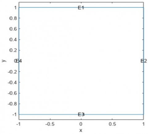
On a square domain, find the solution. This geometry is described by the square g function. Make a model object with geometry included. View the edge labels when creating the geometry (Figure 1).
Figure 1. Using MATLAB to plot edge
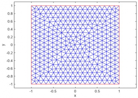
Figure 2. MATLAB code to plot boundary conditions
To determine FEM coefficients, boundary situations on the upper (edge 1), lowest (edge 3), and left (edge 4), as well as right (edge 2) and zero Neumann boundary situation. Then, generate and vision the finite element method for the problem is shown in Figure 2.
2.2 Derivation of the method in one dimension
The below equation outlines a mathematical model describing wave propagation in a specific medium, where the equation captures the behavior of waves within a defined range [-a, a] and is enhanced by boundary conditions that determine the wave's amplitude and behavior at the boundaries. Also, v and w are related to the wave speed and frequency, respectively.
Consider the 1D Helmholtz equation:
$v_{y y}+\frac{w^2}{c(y)^2} v=w g, \quad y \in[-a, a]$ (7)
where, $\left(m_y\right) \subset(-a, a)$ and $m(y)$ and is the frequency as a result are dependent on wave speed.
Based on current objective, Eq. (7) is part of a larger study aiming to improve the accuracy of wave propagation models, particularly at lower frequencies, by considering different approaches like the WKB equation system.
The equation is enhanced by the following boundary conditions:
$\left\{\begin{array}{c}\mathrm{Ķ}_y(-a)-i r \mathrm{Ķ}(-a)=-2 i r B \\ \mathrm{Ķ}_y(a)+\operatorname{irĶ}(a)=0\end{array}\right.$ (8)
where, B is the wave's incoming amplitude. at high frequencies, GO is a good approximation of the answer. We're working on a method to make up for the errors it produces at lower frequencies. The WKB equation system would be the sensible option. However, does not converge even under simple circumstances. There is just an asymptotic sequence. Its limitation to waves travelling in a single direction is a weakness. When c_y0, waves are truly reflected. As a result, we develop the ansatz with two orientations.
The transition from Eq. (7) to boundary conditions (8) involves considering the wave equation vyy+w2c(y)2v=wg in a one-dimensional domain [-a, a].
The boundary conditions are derived by imposing constraints at the boundaries of the domain. At y=-a and y=a, we have: $\mathrm{Ķ} y(-a)-i Ķ(-a)=-2 i B$.
This condition represents how the wave amplitude and its reflection behave at the left boundary (-a).
Ķy(a)+iĶ(a)=0
This condition describes how these quantities behave at the right boundary (a).
These two conditions help define how waves interact with boundaries within this specified range [-a, a], providing crucial insights into their behavior within this confined region.
$\left\{\begin{array}{l}i r v+c(y) v_x-\frac{1}{2} m_y(y) v=g \\ i r v-c(y) v_y-\frac{1}{2} m_y(y) v=g\end{array}\right.$ (9)
where, z=r+v then it satisfies the following equation:
$m^2 z_{y y}+r^2 z=-i r g+\alpha(y) z$ (10)
where,
$\alpha(y)=\frac{1}{2} m m_{y y}-\frac{1}{4} m^2{ }_y$ (11)
Now, we increase the powers of v and w.
$V=\sum_a r_a r^{-a}, W=\sum_a s_a r^{-a}$ (12)
From above equation:
$\begin{aligned} & \sum_a\left(i r r_a+c(x) \partial_y r_a\right)-\frac{1}{2} m_y(y) r_a-\frac{\alpha(y)}{2 i}\left(r_{a-1}+s_{a-1}\right) r^{-a}=0 \\ & \sum_a\left(i r r_a+m(y) \partial_y s_a\right)-\frac{1}{2} m_y(y) s_a-\frac{\alpha(y)}{2 i}\left(r_{a-1}+s_{a-1}\right) m^{-a}=0\end{aligned}$ (13)
Define $v_a=r_a w^{-a}$ and $w_a=s_a w^{-a}$ then get:
$i r r_a-c(y) \partial_y r_a+\frac{1}{2} m(y) r_a=\frac{1}{2 i r} g_a(y)$ (14)
This section explains the numerical solution for Helmholtz equation using finite element method by MATLAB programming where this equation dependent in many electric problems such that it helps the engineering to find variables of different. The Helmholtz problem is resolved using a spectral element solver program developed in MATLAB. The element stiffness matrices and the element mass matrices for the isoperimetric quadrilateral and rectangular elements are assessed to provide steady diffusion and Helmholtz operations with this program.
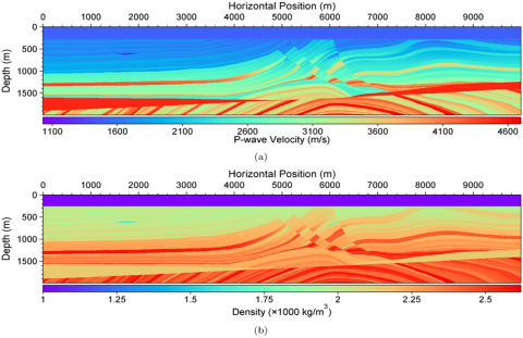
Figure 3. Electric problem model in MATLAB
Researchers must build and validate a new set of Helmholtz equations to solve an electrical problem. After researching the issue, we discovered that each model has significant variances in density and speed. For testing, we contoured the scaled model to have Nz Nx = 400 2000 microelements and to have a horizontal extent of 10 km and a depth of 2 km. Spatial heterogeneity is not impacted by rescaling. The net has a fine mesh size of 5 meters in each direction. To test our FEM-based methodology, we created two different types of course meshes: Mesh 1 includes Nz Nx = 20 100 coarse variables and has a mesh size of 100 m; Mesh 2 includes Nz Nx = 40 200 coarse variables and has a grid size of 50 m. The source lies at a depth of 0.2 km and a horizontal distance of 5 km. Figure 3 shows the electric problem model in MATLAB.
Helmholtz problems with homogeneous or nonhomogeneous Dirichlet and Neumann boundary conditions are resolved using the stable diffusion operator, which is equivalent to the rectangular element stiffness matrix for a single element. The global in order to solve the steady diffusion operators in domains with multiple elements, stiffness matrices made by merging the element stiffness matrices are used. The Helmholtz equation only needs one rectangular element to be solved. The formulas for the Helmholtz operator evaluation are discussed. The use of the Helmholtz equation is demonstrated. Rectangular element formulas are used to evaluate the Helmholtz operator. The results are presented as contour graphs and 3D models. Helmholtz equation with Dirichlet boundary conditions and λ=1.
$\begin{aligned} \frac{\partial^2 v}{\partial x^2}+\frac{\partial^2 v}{\partial y^2}+v & =g \text { on } a \in[-1,1] \times[-1,1] \\ v & =v_{ {exact }} \text { on } \mu\end{aligned}$ (15)
Result in the exact solution of
$v_{{exact }}=\sin (\pi x) \cos (\pi y)$ (16)
by MATLAB version R2021 discussion the result and draw the solution 2D as shown in Figure 4.
Figure 4. Second differential of Helmholtz equation in 2D
To address the scattering problem using the solved function within the general FEM model container framework, one should refer to the electromagnetic workflow that utilizes the Electromagnetic Model in conjunction with a well-established domain-specific language. This setup is crucial for solving the Helmholtz equation effectively. In examining the outcomes, we observe that the solutions manifest as an infinite curve with a definitive endpoint, illustrating the significance and spatial extent of employing the Helmholtz equation. This method is particularly effective in modeling dipole electric functions in physics using the FEM technique.
In a specific scenario involving straightforward scattering, we analyze how incident waves from the left are reflected by a square object. The model considers an infinite horizontal membrane that is slightly displaced vertically, anchored securely at the object's perimeter. Within this homogeneous medium, the phase velocity of the wave remains constant.
The procedure begins by constructing an FEM model centered on a single dependent variable. Following this, the scattering problem is tackled using a programmed approach, and subsequently, the value coefficients are determined. As the analysis progresses, the geometry is transformed, expanding the model where constants have already been defined. Towards the conclusion of this process, one should begin formulating the necessary equations, plot the geometry, and display the edge labels crucial for defining the boundary conditions.
The next step involves applying bounded conditions and solving for the complex amplitude by securing a real-value solution of the Helmholtz equation, which is then stored in the real component of vector u. To visually demonstrate the dynamics of the time-dependent wave equation, an animation is created using the solution derived from the Helmholtz equation as a reference.
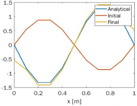
To implement the central difference scheme for the wave equation, a computational program is developed using MATLAB. This scientific programming environment is instrumental in facilitating a deeper understanding of wave behaviors and the impact of boundary conditions on the system.
The number of grid points representing time and space, respectively, is input as sl and sd. If the initial velocity is applied as the initial condition, then R is the right end point of [0, R] Ķm is the right end point of [0, b] Apply as a boundary value but the velocity at the boundary point.
The output v(s, d) the solution and $d s=\frac{s-0}{l s}$ temporal grid size, dĶ= $\frac{b-0}{l s}$, c=0.5, ym=ds/dĶ for j=3:nsns, i=2:nĶ-1. Then, by MATLAB with version R2021 FEM model with a single dependent variable first, then use the programmatic method to address the scattering problem.
The function used to define the geometry provides detailed specifications for the parameters k, c, a, f, where a represents the term with inhomogeneous coefficients.
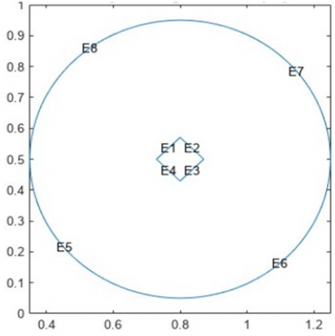
The section Parametrized Function for 2D Geometry Creation in the documentation. the coefficients and the inhomogeneous terms. The geometry should be converted and added to the model. For use in the definition of the boundary conditions, draw the geometry and show the edge figure (Figure 5).
Figure 5. Plot edge of second differential in 3D
Figure 5 refers to a visual representation showing the boundaries or edges of a mathematical model related to the second derivative in a three-dimensional space. This visualization is part of the process of solving the Helmholtz equations using MATLAB and the finite element method, demonstrating the application of computational tools to analyze and solve complex mathematical problems in physics or engineering.
By examining this plot, it can gain insights into how different parameters impact wave propagation and acoustic phenomena within external domains.
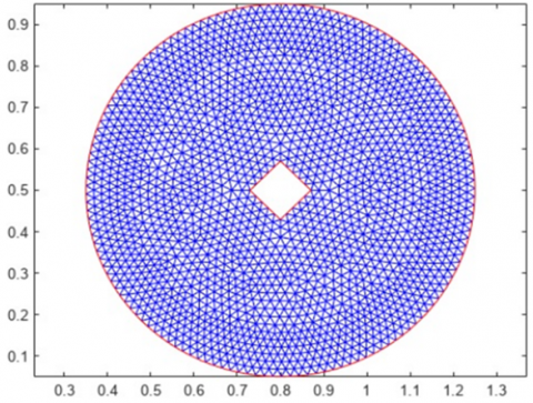
By using the boundary conditions, to determine the coefficients and create a mesh. For this program, we tried to take the extremely small numbers in the interval and the complex numbers from all sides in the form of a circle to be of significant values, so that the analysis would be more accurate. As a result, the shape is as follows as shown in Figure 6.
Figure 6. Plot the second differential equation in 3D
In Figure 6, the plot visualizes the second differential equation in a three-dimensional space. The graph represents the mathematical relationship between the variables in the equation, providing a visual representation of how the equation behaves in a 3D environment. This visualization aids in understanding the behavior and properties of the second differential equation in a more tangible and intuitive way.
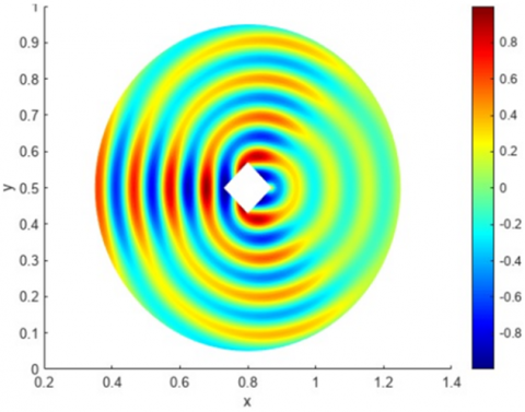
Figure 7. Second differential equation for many points in interval
The complex amplitude should be solved for. The real portion of the vector u contains an approximation to the real value result of the Helmholtz equation. Due to the prior drawing's confusion, the drawing appears (Figure 7) to us in the form that is more generic and correct for Interval because the above drawing only uses a subset of the numbers contained in [1,4,1].
Additionally, Figure 7 provides a visual depiction of the equation's behavior across these points. This visualization aids in understanding the complex amplitude solutions and the accuracy of the Helmholtz equation's real value approximation within the specified interval.
MATLAB R2021 software and the FEM were used in this work to design a spectral element solver program for effectively solving first and second-order Helmholtz equations. To ensure steady diffusion and Helmholtz operations with this program, the element stiffness matrices and the element mass matrices were assessed for the isoperimetric quadrilateral and rectangular elements, giving rise to the development and validation of a new set of Helmholtz equations for solving electrical problems. The derivative variables and their graphical representation were computed to arrive at a reliable solution to complex electrical circuit analysis. Scholars can rely on this study when designing and analyzing electrical circuits that involves deep understanding of derivatives; the importance of computational tools in modern scientific research has also been underscored by the emphasis on developing software tailored to identify key components and represent research outcomes, especially in electrical engineering field. A quick and reliable way of finding solution to the Helmholtz equation in a confined region at varying wave speed functions has also been provided in this work. Even though this work has advanced the capability to model and optimize complex electrical systems, it is important that future studies should aim at the development of parallel algorithms, model reduction methods, or optimization techniques for the improvement of the computational efficiency and accuracy of the system.
[1] Yahya, I.Z.A., Kaedhi, H.M., Karash, E.T., Najm, W.M. (2024). Finite element analysis of the effect of carbon nanotube content on the compressive properties of zirconia nanocomposites. International Journal of Computational Methods and Experimental Measurements, 12(3): 227-235. https://doi.org/10.18280/ijcmem.120304
[2] Parlak, M., Taplak, H. (2020). Rotor-dynamic analysis of a small steam turbine using finite element method. Mathematical Modelling of Engineering Problems, 7(1): 68-72. https://doi.org/10.18280/mmep.070108
[3] Akeremale, C.O., Olaiju, O.A., Yeak, S.H. (2021). H-adaptive finite element methods for 1D stationary high gradient boundary value problems. Mathematical Modelling of Engineering Problems, 8(6): 967-973. https://doi.org/10.18280/mmep.080617
[4] Lyche, T., Merrien, J.L. (2014). Exercises in Computational Mathematics with MATLAB. Springer.
[5] Cheney, E.W., Kincaid, D.R. (2012). Numerical Mathematics and Computing. Monterey County: Cengage Learning, Brooks.
[6] Greenleaf, A., Kurylev, Y., Lassas, M., Uhlmann, G. (2009). Invisibility and inverse problems. Bulletin of the American Mathematical Society, 46(1): 55-97.
[7] Ammari, H., Kang, H., Lee, H., Lim, M. (2013). Enhancement of near-cloaking. Part II: The Helmholtz equation. Communications in Mathematical Physics, 317(2): 485-502. https://doi.org/10.1007/s00220-012-1620-y
[8] Kohn, R.V., Vogelius, M. (1984). Identification of an unknown conductivity by means of measurements at the boundary. In SIAM-AMS Proceedings, pp. 113-123.
[9] Kohn, R.V., Shen, H., Vogelius, M.S., Weinstein, M.I. (2008). Cloaking via change of variables in electric impedance tomography. Inverse Problems, 24(1): 015016. https://doi.org/10.1088/0266-5611/24/1/015016
[10] Schurig, D., Mock, J.J., Justice, B.J., Cummer, S.A., Pendry, J.B., Starr, A.F., Smith, D.R. (2006). Metamaterial electromagnetic cloak at microwave frequencies. Science, 314(5801): 977-980. https://doi.org/10.1126/science.1133628
[11] Mu, L., Wang, J., Ye, X. (2015). A new weak Galerkin finite element method for the Helmholtz equation. IMA Journal of Numerical Analysis, 35(3): 1228-1255. https://doi.org/10.1093/imanum/dru026
[12] Aldirany, Z., Cottereau, R., Laforest, M., Prudhomme, S. (2022). Optimal error analysis of the spectral element method for the 2D homogeneous wave equation. Computers & Mathematics with Applications, 119: 241-256. https://doi.org/10.1016/j.camwa.2022.05.038
[13] Oliveira, S.P., Leite, S.A. (2018). Error analysis of the spectral element method with Gauss–Lobatto–Legendre points for the acoustic wave equation in heterogeneous media. Applied Numerical Mathematics, 129: 39-57. https://doi.org/10.1016/j.apnum.2018.02.007
[14] Rong, Z., Xu, C. (2008). Numerical approximation of acoustic waves by spectral element methods. Applied Numerical Mathematics, 58(7): 999-1016. https://doi.org/10.1016/j.apnum.2007.04.008
[15] Quarteroni, A., Manzoni, A., Vergara, C. (2017). The cardiovascular system: Mathematical modelling, numerical algorithms and clinical applications. Acta Numerica, 26: 365-590. https://doi.org/10.1017/S0962492917000046
[16] Quarteroni, A., Valli, A. (2008). Numerical Approximation of Partial Differential Equations. Springer Science & Business Media.
[17] Hesthaven, J.S., Warburton, T. (2007). Nodal Discontinuous Galerkin Methods: Algorithms, Analysis, and Applications. Springer Science & Business Media.
[18] Rachowicz, W., Zdunek, A. (2005). An hp-adaptive finite element method for scattering problems in computational electromagnetics. International Journal for Numerical Methods in Engineering, 62(9): 1226-1249. https://doi.org/10.1002/nme.1227
[19] Gerstenberger, A., Wall, W.A. (2008). An extended finite element method/Lagrange multiplier based approach for fluid–structure interaction. Computer Methods in Applied Mechanics and Engineering, 197(19-20): 1699-1714. https://doi.org/10.1016/j.cma.2007.07.002