Vimhala Kuppusamy![]() | Lavanya Gowrishankar*
| Lavanya Gowrishankar*![]()
© 2024 The authors. This article is published by IIETA and is licensed under the CC BY 4.0 license (http://creativecommons.org/licenses/by/4.0/).
OPEN ACCESS
This study focuses on mitigating patient congestion in healthcare departments by employing an M/G/1 queue. The system comprises of two crucial servers, HR (Human Resource) and nurse and investigates the flow of patients between them. The HR department's role in managing staffing and generating daily census reports significantly reduces nursing demand and congestion, directing patients to the nursing unit for intensive medical care. The system demonstrates stability when the HR's arrival rate is lower than its service rate, effectively reducing congestion. Utilizing the Matrix-Geometric method ensures system stability, crucial for efficient healthcare operations. The hidden Markov model, supported by the Viterbi algorithm, facilitates the determination of the most efficient HR and nurse sequencing and necessary staffing levels, accommodating sequences of any length. The novelty of the work lies in the choice of Viterbi algorithm in modelling as its computational complexity O(n)=O(6)=O(1). The hidden Markov model and Baum-Welch algorithm offer a comprehensive analysis of patient flow dynamics, unveiling hidden states and transitions that influence system performance. This comprehensive understanding aids in managing overcrowding and optimizing resource utilization. Presenting the results numerically in tables provides a holistic view of healthcare department dynamics, contributing to effective process improvements and resource allocation. This study's innovative integration of methodologies offers a sophisticated approach to understanding and optimizing the dynamics of patient flow in healthcare departments.
matrix-geometric method, patient flow, relative measures, hidden Markov model, Baum-Welch algorithm
Life expectancy at birth continues to increase remarkably throughout the world. With a rise in the mortality age, senior population, expensive new medical technologies, and a society demanding higher quality health care, the demand for optimal cost healthcare is increasing day by day. The population over the age of 65 is rapidly increasing, however longitivity is accompanied with ailments which need due attention. Hospitalizations of elderly patients are more frequent, complicated, carry more risk of being prolonged. All these contribute to added congestion in hospitals leading to the need of proper hospital resource management. Many sections of health care departments face a crisis in both efficient man power and other resource availability. People have been trying to resolve these issues from long by adapting suitable techniques such as having flexi employment of staff and hiring. However, the resource scheduling and management goes a step ahead to resolve these issues for health care providers. In this paper, we provide a queuing model to optimize nurse staffing in a small section of health care unit. This study attempts to provide recommendations and insights that are based on evidence, with the goal of empowering healthcare providers to improve both the quality and efficiency of the treatment they provide to their patients. The goals of the research are framed within the larger framework of enhancing resource allocation, decreasing patient congestion and eventually raising the bar for the quality of treatment provided within healthcare departments.
The M/G/1 model seems to be more appropriate as the arrival patients follows Poisson distribution and require service at various levels consuming different time slots. This leads to a general service pattern. The incoming population needs assistance for direction which is offered by the HR leading to outpatient or admission. In the past, most papers had referred to M/M/1 queues [1, 2]. As the need and time varies from patient-to-patient, general distribution seems to be apt.
Obtaining analytical solutions for the stationary probability of the number of customers in the system for an M/G/1 queue is difficult. Therefore, we use the matrix-geometric method to compute the stationary probability distribution. The matrix-geometric method models and analyses complicated systems with random patient arrivals, service times, and state transitions. It excels in healthcare contexts where patients switch providers and phases of care. Our research will use this strategy to examine if the healthcare department's patient flow system can efficiently manage incoming patients and avoid congestion and delays. The matrix-geometric method investigates complex healthcare unit dynamics by using matrices to express state transition probabilities. It calculates server utilization, patient wait times, and queue lengths. In this work we can provide hospital administrators with data-driven suggestions for nurse staffing and care quality by revealing resource allocation and system efficiency.
The M/G/1 queue is employed and matrix geometric method is used to derive the relative measures. The scenario and conclusions are numerically illustrated and presented as graphs.
1.1 Literature review
Of all the units constituting, a hospital emergency care unit is of at most importance. We shall classify the relevant papers in this review based on their conclusions and the methodology they used, Queueing Theory and Capacity Planning Research: Green [1] addresses this problem of Emergency Department (ED) overcrowding which is a growing problem in current scenario. As some use ED for routine checkups it turns out to be leading to fatal consequences for the seriously ill patients. In this paper the author Linda V Green illustrates how lack of proper capacity management policies by hospital managers and government officials lead to drastic situations. The main cause being mis-understanding of service system dynamics. The queueing system models are employed to identify, rectify and upgrade the existing polices followed for resource allocation, often with negligible additional capacity. Zhang et. al [3] proposed a state dependent model to achieve best possible resource utilization for the benefit of long-term care requirement. Green [2] claimed that queueing analysis has a key role in estimating availability requirements for possible future scenarios, including demand surges due to new diseases or acts of terrorism. This in fact proves useful in handling unanticipated pandemic situations. This work describes basic queueing models as well as some simple modifications and extensions that are particularly useful in the healthcare setting. It is well illustrated by examples showcasing their use. The critical issue of data requirements as well as model choice, model-building is presented. The interpretation of the numerical results well establishes the use of this paper on a day to day basis.
Nurse Scheduling and Workforce Management Research: A new perspective to solving shortage in nurse supply is dealt by Diaz et al. [4]. They have presented a conceptual frame work of nurses’ shortage and have tried to resolve using the industrial solutions. The limitations are also discussed. The nursing shortage has been modelled as a staff scheduling problem using the concept of inventory and queueing theory to optimize the requirement. It is explicitly seen that the simple over-pulling of nurses is generating a fictitious over-demand that is driven by internal demand cycles. In the concluding note it is observed that as per this study the demand at times is common to both the hospital and outside agencies leading to fictitious demand. Healthcare Capacity Management: Fagefors et al. [5] gave an insight to the efficient capacity management in healthcare systems. Overtime, temporary hiring of staff, movement of staff across departments, utilizing external agencies for staff provision and queueing patients and availing the services from external providers have been identified as the major factors contributing towards deficit healthcare staff management. Data collected through questionnaire from the Region Västra Götaland healthcare was used to compute multiple regression analysis. In the end it was found that the prerequisites and required managerial approaches used to efficiently manage most of the capacity in the system differ significantly between different parts of the system. These differences must be addressed. The results in the paper give a clear insight to the shortfalls in capacity management and a clear understanding of efficient capacity management in healthcare systems. Boyle et al. [6] proposed discrete event simulation model for prediction of the impact of delayed discharge in a hospital. The extra time loss for the patients and the denial of beds for the needy patients is considered. Two cases of discharge are discussed wherein patients are moved to smaller community hospitals or sent home with nursing assistance provided by care givers. Simulation model is used in modelling the flow of patients to both intermediate and long-term care in the UK NHS, and modelling delayed discharge using an acceptance probability to represent the situations where a transfer is delayed due to a variety of constraints. This paper is specific to the Southampton context, but could be transformed into a reusable model that can be applied to any hospital. Markov chains and matrix analytic methods in Healthcare Modelling: Latouche and Ramaswami [7] provided an introduction to matrix analytic methods in stochastic modelling, offering foundational insights. Bolch et al. [8] delved into queueing networks and Markov chains, demonstrating their application in modelling healthcare systems. Chakravarthy [9, 10] offered a comprehensive resource on matrix-analytic methods, providing both analytical and simulation approaches in healthcare modelling. Healthcare Quality Assessment Using Hidden Markov Models: Awad et al. [11] introduced hidden Markov models and their potential applications in healthcare, particularly for quality assessment. Mitchell et al. [12] discussed the application of hidden Markov models in capturing the quality of care in geriatric wards, illustrating their practicality in real healthcare scenarios. Apart from the previously described contributions, there exist further applications in the literature that tackle various domains as policy implementation, state-dependent servers, warehouse management, and algorithm-driven learning. Abushilah and Abbas [13] assessed clustering methods and indices using simulated data and R software 3.1, focusing on object group identification and partition optimization. Adiyeloja et al. [14] analysed six brewery plant production lines' efficiency using data envelopment analysis, revealing that two of the most efficient lines required reduced manpower and increased output. Chen and Chen [15] explored a call centre with impatient customers, repairable servers, and Interactive Voice Response Units, highlighting the exponential failure rate and its impact on design parameters.
Saritha et al. [16] examined a single-component inventory model with replenishment schedules, optimizing cost, minimizing service time, and enhancing warehouse stock efficiency. Sama et al. [17] investigated the performance of a two-phase queueing system, utilizing steady state equations and probability generating functions for system design. Jiang et al. [18] proposed reinforcement learning AQM (RLAQM), improving network stability and performance through active queue management. Shah et al. [19] investigated the performance evaluation of a multisatge service system using matrix geometric methods. Through their research, they aim to analyze and assess the efficiency and effectiveness of the system's operation, providing insights into its performance characteristics. Darapaneni et al. [20] explored the performance of MapReduce frameworks using an analytical transient queuing model, examining job arrival rates and completion times. Kumar et al. [21] analyzed a multi-processor call center retrial queueing network, focusing on breakdowns, repairs, and performance measures using matrix-analytic techniques and numerical results.
These studies provide an extending knowledge of queueing theory, capacity planning, healthcare management, and optimization approaches, these works collectively help to improve efficiency and performance across a range of systems and disciplines. The research is primarily focused on M/G/1 queue and matrix-geometric methods, which are fundamental to the research's approach.
As the problem still prevails, we have employed Markov models and M/G/1 queue where in the service requirement each individual patient is different and would not fix to a specific distribution. In Section 2, the model description is discussed, Section 3 depicts the stability condition and stationary distribution of the model. Performance measures are derived in Section 4. Numerical analysis is done in Section 5. Hidden Markov model concept for the observed states is discussed in Section 6 and Section 7 gives the conclusion.
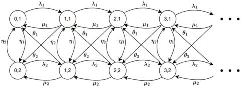
The system under consideration comprises of two states HR and nursing unit namely, assigned to state 1 and state 2 respectively. All arrivals are first directed to the HR for further recommendation of treatment. Patients requiring admission are forwarded to state 2 i.e., the nursing unit. All arrivals pass through HR before reaching nursing unit. λ1 reflects the frequency with which outpatients present to the HR (Human Resources) unit for service. Outpatients are people who come to the healthcare department just for HR services. Consultations, prescription renewals, and recommendations for additional medical care are examples of these services. λ1 is critical in defining the workload of the HR unit. A higher λ1 indicates a greater number of outpatients seeking HR services, affecting HR staff workload and perhaps resulting to longer wait times if not managed properly.
λ2 denotes the rate at which patients requiring admission or inpatient care arrive at the nursing unit. The HR department identifies and refers these patients for more intensive medical treatment and care. The value of λ2 is crucial for determining the demand on the nursing unit. A larger λ2 indicates a bigger number of patients requiring inpatient services, which might constrain resources, affect nursing unit occupancy rates, and impact patient flow within the healthcare department.
The total arrival rate to the healthcare system incorporates both λ1 and λ2, i.e., λ1+λ2. This metric describes the overall patient flow into the healthcare department, including both outpatients and inpatients. The significance of this combined arrival rate resides in its broad impact on the whole healthcare system. It has an impact on the allocation of HR and nursing unit resources, patient wait times, service quality, and overall system efficiency. Understanding and regulating the system arrival rate is critical for optimizing patient care and reducing congestion.
μ1 denotes the transit of the HR from having ‘i’ number of patients to ‘i-1’ number of patients. θ1 denotes the discharge procedure sending a patient by the nurse at state (i, 2) to the HR at (i-1, 1) denoted by N(i, 2)→HR(i-1, 1). The mobility of arriving patients within the states is denoted by "HR to HR" and "nurse to nurse" in the terminology that has been presented in nomenclature. The movement of the patients is defined as (i, 1) to (i+1, 1) and (i, 2) to (i+1, 2) for each possible value of i as in Figure 1. In the given ordered pair, 1 represents HR state and 2 represents nurse state. According to the description, the HR will be responsible for the patient's admission and discharge, during which time the nurse will take over responsibility for the patient's medicine and care. The notations in the table clearly depict the probabilities of the transitions that occur in the proposed model. The limitation for the model is that, the HR sends a patient to nurse only when the number of patients with nurse is less than or equal to that with the HR. Similarly, for transition from nurse to HR.
Figure 1. Transition diagram of patient flow to both HR and nurse
Let N(t) be the number of customers in the system at time t, and ξ(t) be the server states HR and nurse at time t (t≥0). We describe the state space of the proposed model to be {(0, 1), (0, 2)} $\cup$ {(n, i): n≥1, i=1, 2}. The infinitesimal generator Q of the process is given by:
$Q=\left[\begin{array}{cccccc}B & A_0 & . . & . . & . . & . . \\ A_2 & A_1 & A_0 & . . & . & . . \\ . . & A_2 & A_1 & A_0 & . . & . . \\ . . & . . & A_2 & A_1 & A_0 & . . \\ . . & . . & . . & A_2 & A_1 & A_0 \\ . . & . . & . . & . . & . . & . .\end{array}\right]$
where,
$\mathrm{B}=\left[\begin{array}{cc}-\left(\lambda_1+\eta_1\right) & \eta_1 \\ \eta_2 & -\left(\lambda_2+\eta_2\right)\end{array}\right]$,
$A_0=\left[\begin{array}{cc}\lambda_1 & 0 \\ 0 & \lambda_2\end{array}\right]$,
$A_2=\left[\begin{array}{ll}\mu_1 & \theta_2 \\ \theta_1 & \mu_2\end{array}\right]$,
$A_1=\left[\begin{array}{cc}-\left(\lambda_1+\eta_1+\mu_1+\theta_2\right) & \eta_1 \\ \eta_2 & -\left(\lambda_1+\eta_2+\mu_2+\theta_1\right)\end{array}\right]$.
In this section, we look into the mathematical details to thoroughly understand the steady-state behaviour of our healthcare department model. The steady-state analysis is essential in our work as it is a vital metric for determining the efficiency of the system in handling the patient flow. It enables us to assess the stability, performance, and resource allocation of the healthcare system, with the ultimate goal of reducing patient congestion.
3.1 Stability condition
We now derive the condition for the stability of the given queue. Let us define
A=A0+A1+A2.
$\therefore A=\left[\begin{array}{cc}-\left(\theta_2+\eta_1\right) & \theta_2+\eta_1 \\ \theta_1+\eta_2 & -\left(\theta_1+\eta_2\right)\end{array}\right]$.
It can be seen that A is a finite and irreducible generator. There exists a stationary probability vector π=[π0 π1] of A.
For convenience let us denote π0,1=π0, where π0,1 is the steady state transition vector at HR. and π0,2=π1, where π0,2 is the steady state transition vector at nurse.
Also,
$\pi A=0$ and $\pi e=1$ (1)
where, e is the unit column vector.
Using Theorem 3.1.1 in Neuts the necessary and sufficient condition for the stability of the system is as follows:
$\pi A_2 e>\pi A_0 e$ (2)
$-\left(\theta_2+\eta_1\right) \pi_0+\left(\theta_1+\eta_2\right) \pi_1=0$ (3)
$\begin{gathered}\left(\theta_2+\eta_1\right) \pi_0-\left(\theta_1+\eta_2\right) \pi_1=0 \\ \pi_0+\pi_1=1\end{gathered}$ (4)
Solving we get: $\Rightarrow-\left(\theta_2+\eta_1\right) \pi_0-\left(\theta_1+\eta_2\right) \pi_0+\left(\theta_1+\eta_2\right)=0$,
$\pi_0=\frac{\left(\theta_1+\eta_2\right)}{\left(\theta_2+\eta_1\right)+\left(\theta_1+\eta_2\right)}$ (5)
$\pi_1=\frac{\left(\theta_2+\eta_1\right)}{\left(\theta_2+\eta_1\right)+\left(\theta_1+\eta_2\right)}$ (6)
Using $\pi_0$ and $\pi_1$ in inequality (2), we get:
$\rho=\frac{\left(\theta_1+\eta_2\right) \lambda_1+\left(\theta_2+\eta_1\right) \lambda_2}{\left(\theta_1+\eta_2\right)\left(\mu_1+\theta_2\right)+\left(\theta_2+\eta_1\right)\left(\mu_2+\theta_1\right)}<1$ (7)
3.2 Stationary probability distribution
The steady state probability is defined as $P_{i, n}=\lim _{t \rightarrow \infty} \operatorname{Pr}(N(t)=n, \xi(t)=i), n \in N, i=1,2$.
Let π be the stationary probability vector of the generator Q satisfying πQ=0 and πe=1, where 0 is a row vector with all zeros and e is a column vector with all ones. The vector is partitioned as π=[π0, π1, π2, …] where π0=[π0,1, π0,2] and πn=[πn.1, πn.2] for n≥1.
i.e., πne=πn,1+πn,2=1.
Based on the matrix-geometric method [7], the stationary probability vector π can be computed. By applying Lemma 6.4.3 [7] we get the following equations:
$\pi_0\left(B+A_0 G\right)=0$ (8)
$\pi_0(I-R)^{-1} 1=1$ (9)
$\pi_n=\pi_0 R^n, n \geq 1$ (10)
There exist matrices R, U and G satisfying the equations:
$\begin{gathered}U=A_1+A_0 G ; R=A_0(-U)^{-1} ; G=(-U)^{-1} A_2 \\ A_2+G A_1+G^2 A_0=0 ; A_0+R A_1+R^2 A_2=0\end{gathered}$ (11)
The rate matrix R and G are the minimal non-negative solution to the matrix-quadratic equation.
We observe that π0 is the solution of Eq. (8) and the normalizing condition π.e=1 is equivalent to Eq. (9), we have:
$\pi_0 \neq 0 ; B+A_0 G=0$ (12)
From Eq. (12), we can get:
$G=-B A_0^{-1}$ (13)
Substituting Eq. (13) in Eq. (11) we obtain the values of R and U:
$\pi_0=I-R$ (14)
$\pi_1=\pi_0 R$ (15)
Similarly, we can obtain the value of πn for n≥2.
In summary, this section provides a comprehensive analysis of patient distribution and system behaviour using the stationary probability distribution Pi,n , in the healthcare model. The study employs steady-state transition probabilities (π0 and π1) for HR and nurse states. These probabilities are shown by Eqs. (5) and (6) based on system parameters θ and η. The stationary probability vector is computed using the matrix-geometric approach. R, U, and G matrix equations characterize transitions and interactions within the healthcare system. This allows the assessment of system stability and steady-state behaviour [i.e., the stationary probability distribution Pi,n is used in this section to analyze patient distribution and system behaviour in a healthcare model. The proposed model evaluates system stability using matrix-geometric method and steady-state transition probabilities for HR and nurse states.]
The system performance measures are expressed in terms of the stationary probability vector π as follows:
(i) Expected number of customers in the system:
The expected number of customers in the system stands first and foremost priority, because it helps healthcare providers balance the patient population. It is done by understanding the bed requirement and scheduling staff shifts noticing bottlenecks where additional resources should be allotted.
The expected number of customers in the system is given by:
$L_n=\sum_{i=1}^2 \sum_{n=1}^{\infty} n p_{n, i}=\pi_1 e[I-R]^{-2}$ (16)
(ii) Expected number of customers in the queue:
It helps to forecast future patients leads. It serves as a key to estimate capacity requirements for possible future scenarios such as another pandemic or acts of violence (war scenario).
Thus, the expected number of customers in the queue is:
$L_q=\sum_{i=1}^2 \sum_{n=1}^{\infty}(n-1) \cdot p_{n, i}=\pi_1\left[(I-R)^{-2} e-A_2 B^{-1} e\right]-1$ (17)
(iii) Expected waiting time in the system:
The expected waiting time helps us to notify the delays which are the main pot holes leading to sophistication and even death in emergency case treatments. Emergency care plays a vital role for different threatening illnesses, accident cases, bleeding, breathing difficulties and epileptic seizures. This could be addressed and minimized only if the expected waiting time is taken into account. The expected waiting time in the system is:
$W_s=\frac{L_s}{\lambda_1+\lambda_2}$ (18)
(iv) Expected waiting time in the queue:
The waiting time in the queue is the very important determining factor for quality patient experience. It directly measures the level of care one receives. It is a major challenge faced by big hospitals throughout the country. Increased waiting time is a cause of stress for both the patient and doctor so needs attention.
Hence, the expected waiting time in the queue is found to be:
$W_q=\frac{L_q}{\lambda_1+\lambda_2}$ (19)
To numerically demonstrate how the system performance measures behave under different system parameters, Mat lab software was used. The queueing system's parameters are first defined in the code. The arrival rates of two different customer types (outpatient and inpatient) are shown by λ1 and λ2. The MGM model's parameters are represented by the matrices A2, A1, A0, and B. The parameter values for the model are listed in Table 1. Based on these values, the transition matrices π0 and π1 are derived using the matrix computations A, D, G, U, and R. Additionally, performance indicators for system utilization and customer wait times are captured using Mat lab code. All system parameters are chosen in a way so that they satisfy the stability condition ρ<1.
Table 1. Values of parameter used in the model
|
(λ1, λ2) |
(μ1, μ2) |
(η1, η2) |
(θ1, θ2) |
|
(21,12) |
(25,14) |
(0.5, 0.4) |
(0.4,0.3) |
Table 2. Arrival rates and system performance measures
|
(λ1, λ2) |
Ln |
Lq |
Ws |
Wq |
|
(15,10) |
1.4563 2.2727 |
0.8720 1.5719 |
0.0583 0.0909 |
0.0349 0.0629 |
|
(15,11) |
1.4563 3.2353 |
0.8697 2.4676 |
0.0560 0.1244 |
0.0334 0.0949 |
|
(15,12) |
1.4563 5.0000 |
0.8677 4.1648 |
0.0539 0.1852 |
0.0321 0.1543 |
|
(15,13) |
1.4563 9.2857 |
0.8661 8.3822 |
0.0520 0.3316 |
0.0309 0.2994 |
|
(15,14) |
1.4563 35.0000 |
0.8647 34.0277 |
0.0502 1.2069 |
0.0298 1.1734 |
|
(17,10) |
2.0482 2.2727 |
1.3851 1.5703 |
0.0759 0.0842 |
0.0513 0.0582 |
|
(19,10) |
3.0159 2.2727 |
2.2729 1.5691 |
0.1040 0.0784 |
0.0784 0.0541 |
|
(21,10) |
4.8837 2.2727 |
4.0599 1.5681 |
0.1575 0.0733 |
0.1310 0.0506 |
|
(23,10) |
10.0000 2.2727 |
9.0946 1.5673 |
0.3030 0.0689 |
0.2756 0.0475 |
|
(25,10) |
83.3333 2.2727 |
82.3457 1.5666 |
2.3810 0.0649 |
2.3527 0.0448 |
Table 2 shows that, when λ1 and λ2 approach μ1 and μ2 respectively, there is a steep increase in the number of customers in the system. When λ1<μ1 and λ2<μ2 , the system gives an optimal number of customers with a moderate gradient. If the number of patients assigned to nursing unit is constant the relative measures do not increase drastically as far as λi<μi, i=1, 2. This is observed for all measures Ln, Lq, Ws, Wq.
(a)
(b)
Figure 2. (a) Performance measures for fixed λ1(15) and varying λ2; (b) Performance measures for fixed λ2(10) and varying λ1
As the number of customers in the system increases, the waiting time in the queue and the system proportionally increase. This would help to manage the resources, avoiding congestion. The moderate gradient as seen from the graph depicts efficient functioning of the system avoiding too much congestion after λ2 reaches 13 (in Figure 2(a)) and λ1 reaches 23 (in Figure 2 (b)) the steep rise in the slope suggests a proportional increase in the patient population. This is observed for all the measures. The last scenario gives the most preferrable condition in healthcare management. However, in real time the previous 2 scenarios are more in vogue. This leads to the study of congestion analysis time after time though previous literature is available. The data in Table 2 has been illustrated using the following two graphs. When λ1 is fixed the rate of change is observed and studied for HR. In this case the system is stable up to a population size of 13 when λ1=15. When λ2 is fixed the rate of change is observed and studied with respect to nurse utilization the HR component being stable. From the graph depicted below it is clearly seen the system is very efficient up to a patient population of 23 when λ2=10. This indicates that λ1 and λ2 play a crucial role in the stability of the system based on μ1 and μ2. Therefore, it is essential to optimize the cost and at the same time increase μ1 and μ2 to the maximum possible extent. This would help to increase the system capacity without affecting its cost effective functioning.
In the context of a hospital patient flow model, HR job is to collect the data or medical records of patient, scheduling appointment and billing the amount for taking care of patients. Nurses job is to escort the patient to the bed, checking patient health and needs, help the doctor in emergency situation. Here adding an inpatient denotes an admission and reduction of inpatient or sending an inpatient back to HR denotes a discharge. The hidden states are HR and nurse as the Human Resources and nursing states describe the internal procedures and operations of the healthcare system. External observers or patients cannot directly observe these states. Admission and discharge states, on the other hand, are visible because they correspond to actual interactions patients experience with the healthcare system. Patients can see when they are admitted or discharged, but they often do not have direct access to HR or nurse processes. Moreover, the distribution of resources, such as staff scheduling and resource management, takes place predominantly in the HR and nurse states. These internal decisions have an impact on the flow of patients between admission and discharge. As a result, it is critical to treat HR and nurse states as hidden since they influence observed states but are not directly evident to patients.
Hospital has to know, whether the service provided by nurse and HR are good but they are hidden. So, by admission and discharge which is discussed in the hidden Markov model (HMM) finds application in forecasting both admission and discharge sequences. A hidden Markov model (HMM) consists of two parts: hidden and observed elements. The hidden part, governed by a Markov process, remains unobserved, while the observed part depends on the hidden part's realization. Analyzing a recorded sequence of events allows in identifying hidden states and understanding the relationship between the components.
In the following discussion, we examine a discrete output hidden Markov model, where the hidden component is characterized by a homogeneous Markov chain.
·H={HR, N} a set of h(=2) hidden states; where HR denotes HR nurse and N denotes nurse in the bed system.
·O={A, D} a set of m(=2) observed states; A denotes admission to bed and D denotes discharge from bed.
·π=(πHR, πN) initial distribution, where $\pi_i \stackrel{\text { def }}{=} \pi_{H_i}=P\left(X_0=H_i\right) \geq 0$;
·P=[pij], 1≤i, j≤2, transition probability matrix between the hidden states HR and nurse. i.e., $P=P\left(X_t=N \mid X_{t-1}=H R\right)$ for a hidden random variable Xt with H states in total.
·E=[eij], output probability or the emission matrix, i.e., the probability of observing A or D at time t for state Xt=N is given by, $E=P\left(Y_t=A\right.$ or $\left.D \mid X_t=N\right)$.
The elements of the transition matrix and the emission probability satisfy the following conditions $\sum_{j=1}^h p_{i j}=1, \sum_{j=1}^m e_{i j}=1$ and the initial distribution π satisfy the condition $\sum_{j=1}^h \pi_j=1$.
Thus, we can describe a hidden Markov chain by θ=(P, E, π). The objective is to deduce the concealed states responsible for generating specific observed sequences or predict forthcoming observations and hidden states using available data. Accomplishing this task is typically achieved through algorithmic approaches such as the Forward-Backward algorithm, Viterbi algorithm, or Baum-Welch algorithm, all of which enable efficient computation of probabilities and likelihoods linked to the hidden states.
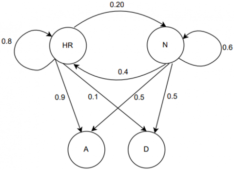
To depict the dynamics of hidden states, we shall establish a random initialization of a probability matrix indicating the transitions between these states. The relationships between hidden states, is represented in Figure 3.
Figure 3. Transition diagram for hidden states
It is necessary to have the parameters P, E, and π in order to accurately characterize the HMM. One of the most important requirements for these parameters is that they should fulfill the normalization constraints, which ensure that the probabilities add up to 1. The purpose of our model is to make use of these parameters (θ) to either infer the hidden states (HR and nurse) that are accountable for the generation of particular observable sequences (admission and discharge) or make predictions about upcoming observations and hidden states. This is done by making use of the data that is currently accessible. This is accomplished using the Baum-Welch algorithm, which provides assistance in estimating the values of the parameters P, E and π in our scenario. The Baum-Welch algorithm’s goal is to locate the local maximum of the likelihood function, which represents the probability of the observed data (A and D) given by the HMM parameters. This local maximum can be thought of as the best possible estimate of the probability of the observed data. This estimation is performed based on the sequences that have been observed, and it enables you to infer the hidden states that are most likely to be present, as well as the transitions between them.
We shall now assume the starting values of HR and nurse as π=[0.4 0.6]. Applying Baum-Welch algorithm for the random initial conditions set above in Figure 3, we can find the local maximum for $\theta^*=\operatorname{argmax}_\theta P(O \mid \theta)$ (i.e., the HMM parameters θ that maximize the probability of the observation) and the expected transition count.
Table 3. Output results from the Baum-Welch Algorithm for the Hidden Markov Model (HMM) parameter estimation based on the observation sequence ADADDA
|
|
Expected Transition Count |
Expected Emission Count |
||
|
HR |
N |
A |
D |
|
|
HR |
2.0988 |
0.7356 |
1.4545 |
1.5455 |
|
N |
0.7123 |
1.4533 |
1.5000 |
1.5000 |
|
|
Normalized Transition Matrix |
Normalized Emission Matrix |
||
|
HR |
N |
A |
D |
|
|
HR |
0.7466 |
0.3360 |
0.4923 |
0.5075 |
|
N |
0.2534 |
0.6640 |
0.5077 |
0.4925 |
As an example, we examine a sequence of observations, denoted as “ADADDA,” with a length of six. MATLAB software was utilized to calculate the expected transition count, emission count, estimated transition matrix, and emission matrix. The resulting output is presented in the Table 3.
Figure 4. Probability distribution related to hidden states
Figure 4 illustrates that the likelihood of a specific observed state occurring varies based on the corresponding hidden state. The probabilities of transitioning from the state HR to discharge are slightly higher compared to transition to the admission state. When the hidden states are HR and nurse, the admission and discharge processes exhibit equally likely occurrence with slightly varying probability.
Viterbi algorithm
Step 1: Initialization.
Initialize the variables Viterbi path, state paths, and state probabilities, the initial observation (in this case, "A"), with t=1.
Step 2: Initialization of the First Observation
HR and nurse for each concealed state:
Determine the probability of the starting state: HR*E(A|HR)=δt(HR).
where δt is used to denote the probability of being in a particular state at a specific time point in the sequence of observations.
Determine the probability of the starting state: nurse is equal to nurse * E(A|nurse).
Step 3: Recursion
The following observations (in this case, "D," "A," "D," "D," "A") follow HR and nurse for each concealed state:
Based on the maximum of the probability of the previous state and the likelihood of the transition, determine the state probability:
Max($\delta_t$(nurse) * P(HR|nurse) * E(D|HR), $\delta_t$ (HR) = $\delta_{t-1}$ (nurse) * P(HR|nurse) * E(D|HR)).
Nurse=max (nurse-1(HR) * P(nurse|HR) * E(D|nurse), nurse-1(nurse) * P(nurse|nurse) * E(D|nurse)).
For each concealed state (HR and nurse), note the most likely prior state.
Step 4: Finishing
Determine the latest observation's highest state probability:
P*(last) is equal to max(δT(HR), δT (nurse)), where T is the sequence's length and δT corresponds to the probability of being in a specific state at the end of the observed sequence.
Step 5: Turning around
Backtrack through the state routes ($\psi$), starting with the most likely state in the previous observation (HR or nurse), to determine the best route for the entire sequence.
Every time step t (from T-1 to 1):
Pick the concealed state with the prior state which the recorded pathways indicate was the most likely.
Step 6: Ending
Taking into account the estimated transition probabilities and emissions for the HR and nurse states, the Viterbi path (π) now provides the most advantageous course for the observed sequence ("ADADDA").
Based on the probabilities provided by the Baum-Welch algorithm, the Viterbi algorithm aids in determining the most probable sequence of hidden states (HR and nurse) which produced the observed sequence ("ADADDA"). When analyzing hidden state dynamics in healthcare contexts, the resulting Viterbi path is a crucial tool.
Subsequently, we employ the Viterbi algorithm to determine the optimal path of the observed sequence, utilizing the transition matrix obtained through Baum-Welch algorithm.
From Figure 5, the optimal Viterbi path is seen to be HR-N-HR-N-N-HR with the emission sequence of A-D-A-D-D-A.
Figure 5. Optimal path for sequence of length six
An M/G/1 queuing model is proposed to break down a healthcare system's complex patient flow into HR and nurse states in this investigation. Patient backflow is common in healthcare operations, so we've allowed it. The relative measures are calculated using the matrix-geometric approach to assess system performance under different scenarios. In this study it is found that the system is stable when the arrival rate of patients seeking HR assistance (λ1) is lower than the HR service rate (μ1). Healthcare administrators should note that HR remains stable while patient numbers rise. Our study digs deeper, especially when admission levels shift. Table 2 shows a considerable increase in relative measures when the admission rate (λ) approaches the service rate (μ). This observation is notable since it shows that HR system efficiency reduces more than nurse unit efficiency when patient arrivals rise. Healthcare administrators need this information to understand how operational scenarios affect patient congestion and system performance. To guarantee efficient patient care during high admission periods, staffing and resource allocation must be effective. Hidden Markov is used to enhance the analysis. Future admission and discharge sequences can be forecasted and one could find the best paths using this method. This forecasting can transform healthcare management to its best. It helps decision-makers distribute resources, manage patient loads, and improve healthcare delivery. Our analysis and the Hidden Markov technique are both academically and practically useful. They help healthcare executives make data-driven decisions to reduce patient congestion and maintain high-quality care.
|
λ1 |
Arrival rate to HR from HR |
|
μ1 |
Service rate from HR to HR |
|
λ2 |
Arrival rate from nurse to nurse |
|
μ2 |
Service rate from nurse to nurse |
|
η1 θ2 |
Arrival rate from HR to nurse (state 1 to state 2) HR(i,1) $\rightarrow$ N(i,2) HR(i,1) $\rightarrow$ N(i-1,2) |
|
θ2+η1 |
Arrival rate from HR to nurse |
|
η2 θ1 |
Arrival rate from nurse to HR (state 2 to state 1) N(i,2) $\rightarrow$ HR(i,1) N(i,2) $\rightarrow$ HR(i-1,1) |
|
θ1+η2 |
Arrival rate from nurse to HR |
[1] Green, L.V. (2010). Using queueing theory to alleviate emergency department overcrowding. Wiley Encyclopedia of Operations Research and Management Science. https://doi.org/10.1002/9780470400531.eorms0987
[2] Green, L. (2006). Queueing analysis in healthcare. Patient Flow: Reducing Delay in Healthcare Delivery, 281-307. https://doi.org/10.1007/978-0-387-33636-7_10
[3] Zhang, Y., Puterman, M.L., Nelson, M., Atkins, D. (2012). A simulation optimization approach to long-term care capacity planning. Operations Research, 60(2): 249-261. https://doi.org/10.1287/opre.1110.1026
[4] Diaz, D.M., Erkoc, M., Asfour, S.S., Baker, E.K. (2010). New ways of thinking about nurse scheduling. Journal of Advances in Management Research, 7(1): 76-93. https://doi.org/10.1108/09727981011042865
[5] Fagefors, C., Lantz, B., Rosén, P. (2020). Creating short-term volume flexibility in healthcare capacity management. International Journal of Environmental Research and Public Health, 17(22): 8514. https://doi.org/10.3390/ijerph17228514
[6] Boyle, L.M., Currie, C.S., Fernandez, C.L., Nguyen, L., Halpenny, C. (2023). A discrete event simulation model of a hospital for prediction of the impact of delayed discharge. In Proceedings of the Operational Research Society Simulation Workshop 2023, Southampton, United Kingdom. https://doi.org/10.36819/SW23.029
[7] Latouche, G., Ramaswami, V. (1999). Introduction to matrix analytic methods in stochastic modeling. Society for Industrial and Applied Mathematics. https://doi.org/10.1137/1.9780898719734
[8] Bolch, G., Greiner, S., De Meer, H., Trivedi, K.S. (2006). Queueing Networks and Markov Chains: Modeling and Performance Evaluation with Computer Science Applications. John Wiley & Sons. https://doi.org/10.1002/0471791571
[9] Chakravarthy, S.R. (2022). Introduction to Matrix-Analytic Methods in Queues 2: Analytical and Simulation Approach-Queues and Simulation. John Wiley & Sons. https://doi.org/10.1002/9781394165421
[10] Chakravarthy, S.R. (2022). Introduction to Matrix-Analytic Methods in Queues 2: Analytical and Simulation Approach-Queues and Simulation. John Wiley & Sons. https://doi.org/10.1002/9781394174201
[11] Awad, M., Khanna, R., Awad, M., Khanna, R. (2015). Hidden Markov model. Efficient Learning Machines: Theories, Concepts, and Applications for Engineers and System Designers, 81-104. https://doi.org/10.1007/978-1-4302-5990-9
[12] Mitchell, H., Marshall, A.H., Zenga, M. (2015). Using the hidden Markov model to capture quality of care in Lombardy geriatric wards. Operations Research for Health Care, 7: 103-110. https://doi.org/10.1016/j.orhc.2015.06.003
[13] Abushilah, S.F., Abbas, R.H. (2023). Performance evaluation of some clustering algorithms under different validity indices. Mathematical Modelling of Engineering Problems, 10(4): 1271-1280. https://doi.org/10.18280/mmep.100420
[14] Adiyeloja, I., Kehinde, O., Babaremu, K., Jen, T.C., Okokpujie, I. (2023). Performance evaluation of production lines in a manufacturing company using data envelopment analysis (DEA). Mathematical Modelling of Engineering Problems, 10(1): 39-47. https://doi.org/10.18280/mmep.100105
[15] Chen, P.S., Chen, Y. (2017). Analysis of a call center with impatient customers and repairable server. Advances in Modelling and Analysis A, 54(1): 142-150. https://doi.org/10.18280/ama_a.540110
[16] Saritha, S., Mamatha, E., Reddy, C.S. (2019). Performance measures of online warehouse service system with replenishment policy. Journal Européen des Systèmes Automatisés, 52(6): 631-638. https://doi.org/10.18280/jesa.520611
[17] Sama, H.R., Vemuri, V.K., Talagadadeevi, S.R., Bhavirisetti, S.K. (2019). Analysis of an N-policy MX/M/1 two-phase queueing system with state-dependent arrival rates and unreliable server. Ingénierie des Systèmes d’Information, 24(3): 233-240. https://doi.org/10.18280/isi.240302
[18] Jiang, F.C., Feng, C.W., Zhu, C., Sun, Y. (2020). Performance analysis of active queue management algorithm based on reinforcement learning. Journal Européen des Systèmes Automatisés, 53(5): 637-644. https://doi.org/10.18280/jesa.530506
[19] Shah, Wajiha, Syed Asif Ali Shah, Safeeullah Soomro, Farrukh Zeeshan Khan, and Gordhan Das Menghwar. Performance evaluation of multisatge service system using matrix geometric method. In 2009 Fourth International Conference on Systems and Networks Communications, Porto, Portugal, pp. 265-269. IEEE, 2009. https://doi.org/10.1109/ICSNC.2009.100
[20] Darapaneni, C.S., Rao, B.B., Satya Vara Prasad, B.B.V., Bulla, S. (2021). An analytical performance evaluation of MapReduce model using transient queuing model. Advances in Modelling and Analysis B, 64(1-4): 46-53. https://doi.org/10.18280/ama_b.641-407
[21] Kumar, B.K., Sankar, R., Krishnan, R.N., Rukmani, R. (2022). Performance analysis of multi-processor two-stage tandem call center retrial queues with non-reliable processors. Methodology and Computing in Applied Probability, 24: 95-142. https://doi.org/10.1007/s11009-020-09842-6