Fatina Shukur*![]() | Safaa Jasim Mosa
| Safaa Jasim Mosa![]() | Kamal M.H. Raheem
| Kamal M.H. Raheem![]()
© 2024 The authors. This article is published by IIETA and is licensed under the CC BY 4.0 license (http://creativecommons.org/licenses/by/4.0/).
OPEN ACCESS
In this research, a new control technique based Fuzzy-PD and Back-Propagation Neural Network is developed for controlling robotics arm with their three links. The continuous modification of the overlapping rate of the membership function improved the efficiency of traditional Fuzzy-PD when compound with the use of Neural Network with Back-Propagation. Initially, the overlapped rate is defined as the amount of the intersecting point of two neighboring membership functions. The integration of Fuzzy-PD and Back-Propagation Neural Network offers a hybrid control system that combines the robustness and interpretability of fuzzy logic with the adaptability and learning capabilities of neural networks. This approach can lead to improve control performance and enhance system behavior in various real-world applications. Then, the overlapped percentage is optimized online using Neural Network with Back-Propagation. The "overlapping rate of the membership function" is a key aspect of fuzzy logic systems. In fuzzy logic, membership functions convert input data into linguistic variables for decision-making. These functions determine the degree of membership of an element in a fuzzy set, ranging from 0 to 1. The overlapping rate refers to how much membership functions of different fuzzy sets intersect with each other. By adjusting this rate, we control the level of ambiguity in the system's decisions. Higher overlapping rates result in smoother transitions between fuzzy sets, allowing for more flexible and tolerant decision boundaries. On the other hand, lower overlapping rates create sharper boundaries, leading to more distinct and precise distinctions between fuzzy sets. Selecting the appropriate overlapping rate is crucial for designing an effective fuzzy logic system. We run a set of experiments to evaluate our proposed method. The final outcomes demonstrate the usefulness and efficiency of our approach and modeling using a 3-DOF robotics arm. When the suggested Fuzzy-PD based on Back-Propagation Neural Network approach is compared to the conventional F-PD technique, we found that the suggested approach is quicker, with a 25% shorter time with an overrun of 0.006m, whereas the F-PD technique has an overshoot less than 0.01m. and reduces overshoot by 49.1%.
3-DOF robotics arm, Fuzzy-PD, membership function, neural network
Robotics manipulators play an important role within a human daily-life activity. Due to their flexible deployments in various domains, they offer a wide range of usage in different applications. These include industry production, surgical intervention, space explorations and military operations. In real-world applications, the robotics arm should essentially trace a defined manifold, which are required to determine an accurate position control [1]. Robotic arms have multiple joints and links, making their kinematics complex. Accurate motion planning is required to ensure the end effector (gripper) reaches its intended position and orientation. Inverse kinematics, which involves finding joint angles to achieve a desired end effector pose, can be particularly challenging. Controlling the robotic arm's movements requires considering its dynamic behavior, including inertia, gravity, and friction. Developing robust control algorithms to account for these factors ensures smooth and accurate motion execution. Controlling a robotic arm can be challenging due to several factors like:
The traditional Proportion-Integration-Differentiation (PID) control approach has evolved and been combined with a developed control method, with several applications in robotic controls [2, 3]. Because of adjusting control improvement consumes time and it depends on user’s experience, an advanced control system should be linked with PID to give an intelligent control gain adjustment. Xiong and Liu [4] studied that traditional PID can be combined with Neural Network so that it learns the best fitting parameters. Fuzzy Logic is usually used to optimize the control gains of classical PID due to the benefits of fuzzification mechanism [5-9]. Fuzzification, defuzzification, and fuzzy reasoning are common components of Fuzzy Logic [10-14]. As the link between traditional crisp and fuzzy arithmetic, the Membership Function (MF) is considered the main part in this procedure. According to the main design of the Fuzzy Logic concept, the fundamental of logical function is to discover the best membership function and fuzzy inference approaches. Therefore, there is not a conventional procedure for transforming people's experience or understanding the fuzzy rules or add something to keep consistency of a fuzzy logic system while constructing such system. In addition to building dataset while constructing fuzzy Logic system. This is the fundamental challenge of fuzzy logic system design. Moreover, researchers define membership function clearly without enhancing the effectiveness of reasonability [14-18]. When designing a membership function, the following issues should be taken into consideration:
Which number of membership function should be used?
Which membership function form should be chosen?
How much every neighboring membership function should intersect?
It is critical to develop a technique of membership function of digital training and calibrating, such that we could successfully get an ideal and optimum system's efficiency.
The acquiring and training of membership function with fuzzy rules are, in fact, the most essential and challenging tasks in designing the architecture of Fuzzy Logic methods for actual control systems [19-21]. There is not entirely dependable and methodical approach that has been discovered yet. In fact, this is a significant limitation of Fuzzy Logic control when deploy it in a practical application. As a result, for experiments and simulation, the technique that is suggested in this research is depending on the PD controller. Hence, we present a novel method FUZZY-PD based on Back-Propagation Neural Network, such that it is used to improve the effectiveness of F-PD even more. Consequently, three criteria are specified for the whole formulation of membership function. These are: Amount of Membership Function (QMF), Shapes of Membership Function (SMF), and Overlapping Rate of Membership Function (ORMF). These functions, however, are associated with the three issues listed above.
The relationship between the control efficiency and overlaying rate will be investigated in this research.
Our goal is to get the optimal overlaying rate, where Neural Network with Back-Propagation are used to optimize the membership function variables. In addition, simulations and practical tests with a 3-DOF robot manipulators are used to show the control strategy. The rest of the paper is structured as follows. Section 2 describes the robotics manipulator with 3-chain links. Section 3 presents the standard F-PD design procedure. Section 4 explains the Neural Network with Back-Propagation technology. Section 5 illustrates our proposed model and experimental results. Finally, Section 6 shows conclusions with our future directions. Upon comparing the suggested Fuzzy-PD based on Back-Propagation Neural Network approach with the conventional F-PD technique, we observed that the former demonstrates improved efficiency, completing the task 25% faster. On the other hand, the latter technique displays an overshoot and successfully achieves a 50% reduction in overshoot.
The kinematics of the 3-DOF robot arm have two major issues: the first is forwards kinematics, and the second is inverse kinematics. Dynamic formulas of the 3-DOF RRR robot manipulators are a collection of mathematical formulas that explain the dynamic characteristics of the robot [3-5]. Forward and inverse kinematics are two fundamental concepts used to describe the motion of a robotic manipulator, such as a 3-DOF (Degrees of Freedom) robotic arm.
Forward Kinematics
Forward kinematics deals with determining the position and orientation of the robot's end effector (e.g., gripper or tool) based on the joint angles or displacements of the robot's links. It essentially answers the question, "Where is the end effector located in the workspace given the joint angles?"
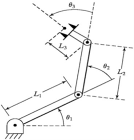
For a 3-DOF robotic manipulator, the forward kinematics problem involves finding the transformation matrix that maps the joint space to the Cartesian space. The transformation matrix consists of rotation and translation components, representing the end effector's position and orientation relative to a fixed reference frame. The system comprises three masses, denoted as m1, m2, and m3, interconnected by weightless links of lengths L1, L2, and L3. The angles of these links are represented by q1, q2, and q3, respectively. To describe the manipulator kinematics, the Denavit-Hartenberg (DH) notation [3] is employed. Table 1 provides the arm parameters for the 3R robot.
Table 1. 3-DOF robot DH parameters
|
Joint No. |
$\boldsymbol{\theta}_i$ |
$\alpha_{\mathrm{i}-1}$ |
di |
ai-1 |
|
1 |
q1 |
0 |
0 |
0 |
|
2 |
q2 |
0 |
0 |
L1 |
|
3 |
q3 |
0 |
0 |
L2 |
|
4 |
0 |
0 |
0 |
L3 |
Each link of the 3-DOF robot manipulator will have its corresponding Transformation Matrix (T.M.) [6]:
${ }_1^0 T=\left[\begin{array}{cccc}C_1 & -S_1 & 0 & 0 \\ S_1 & C_1 & 0 & 0 \\ 0 & 0 & 1 & 0 \\ 0 & 0 & 0 & 1\end{array}\right]$ (1)
${ }_2^1 T=\left[\begin{array}{cccc}C_2 & -S_2 & 0 & L_1 \\ S_2 & C_2 & 0 & 0 \\ 0 & 0 & 1 & 0 \\ 0 & 0 & 0 & 1\end{array}\right]$ (2)
${ }_2^3 T=\left[\begin{array}{cccc}C_3 & -S_3 & 0 & L_2 \\ S_3 & C_3 & 0 & 0 \\ 0 & 0 & 1 & 0 \\ 0 & 0 & 0 & 1\end{array}\right]$ (3)
${ }_4^3 T=\left[\begin{array}{cccc}1 & 0 & 0 & L_3 \\ 0 & 1 & 0 & 0 \\ 0 & 0 & 1 & 0 \\ 0 & 0 & 0 & 1\end{array}\right]$ (4)
So, the tip of end effector transformation to the base will be [3, 4]:
${ }_0^4 T=\left[\begin{array}{cccc}C_{123} & -S_{123} & 0 & L_3 C_{123}+L_2 C_{12}+L_1 C_1 \\ S_{123} & C_{123} & 0 & L_3 S_{123}+L_2 S_{12}+L_1 S_1 \\ 0 & 0 & 1 & 0 \\ 0 & 0 & 0 & 1\end{array}\right]$ (5)
This research is focused on the kinematics of a 3-DOF robot manipulator. The dynamic of the robot has two challenges. The first challenge, which is called forward kinematics, is given a tracking path, location, velocity, and acceleration. Then, it should identify the appropriate torque for each joint to rotate the link connected to it by a certain angle in order to reach the target. While the second challenge is the mechanism of movement with torque set to determine the location, velocity, and acceleration of the robot. The dynamic Eq. may be used to operate the robotic arms. The control challenge consists of developing manipulator dynamic models and using these methods to accomplish the required system performance and responsiveness. Researchers in studies [3, 4, 10] discussed the dynamic model of the robotic system. Figure 1 shows a simple 3-DOF serial robotic manipulator model of a 3-links robot arm [3].
Figure 1. 3-DOF robot manipulator
Inverse Kinematics
Inverse kinematics, on the other hand, involves determining the joint angles or displacements needed to achieve a desired position and orientation of the end effector in the workspace. In other words, it answers the question, "What joint angles do I need to set to reach a specific point in the workspace?" Finding the inverse kinematics solution can be more challenging than forward kinematics, especially for complex robotic arms with multiple degrees of freedom. For a 3-DOF robot, the inverse kinematics problem requires solving a set of trigonometric equations to calculate the joint angles.
The solution to inverse kinematics is not always unique, and multiple configurations may exist to reach a given end effector position. In some cases, certain joint configurations may be physically infeasible due to constraints in the robot's design. Solving the inverse kinematics problem is essential for tasks such as trajectory planning, path following, and object manipulation, as it allows the robot to reach specific points in space accurately and efficiently.
Both forward and inverse kinematics are fundamental tools in robotic manipulator control and play a vital role in various applications, from pick-and-place operations in manufacturing to robotic arm motion planning in diverse industries.
The Lagrangian dynamics formulation provides a means to derive the equations of motion by utilizing a function known as the Lagrangian. This function is defined as the difference between two types of energy: kinetic and potential energy. For the given system, the Lagrangian can be expressed as follows:
$E_{(\theta, \dot{\theta})}=k_{(\theta, \dot{\theta})}-u_{(\theta)}$ (6)
$E_{(\theta, \dot{\theta})}=\frac{1}{2} m * v_c^2(\theta, \dot{\theta})$ (7)
The robot kinematic equation is as follows:
$\tau=M_{(q)} \ddot{q}+V_{(q, \dot{q})}+G_{(q)}$ (8)
$\boldsymbol{G}_{(\boldsymbol{q})}$ is 3×1 vector of gravity
$\boldsymbol{V}_{(\boldsymbol{q}, \dot{\boldsymbol{q}})}$ is 3×1 vector of Coriolis and centrifugal
$\boldsymbol{M}_{(\boldsymbol{q})}$ is 3×3 mass matrix
F-PD models, also known as Fuzzy-PID models, are an extension of traditional PID (Proportional-Integral-Derivative) controllers used in control systems. PID controllers are widely employed in various industrial and engineering applications to regulate processes by adjusting a control signal based on the error between the desired setpoint and the actual process variable. F-PD models integrate fuzzy logic principles into the PID control framework, enhancing the controller's adaptability and performance in dealing with non-linear and uncertain systems. By incorporating fuzzy logic, which allows the representation of linguistic variables and expert knowledge, F-PD models can handle imprecise and uncertain information more effectively.
Fuzzy logic is a mathematical approach that deals with uncertainty by permitting degrees of membership instead of strict binary values. Unlike classical logic, which relies on "true" or "false" conditions, fuzzy logic allows intermediate truth values between 0 and 1, representing the degree of membership of an element in a particular set.
In fuzzy logic, variables are defined linguistically using fuzzy sets, and control rules are expressed in the form of IF-THEN statements based on these fuzzy sets. These rules enable the control system to make decisions or adjust actions based on the input conditions, even in the presence of imprecise or ambiguous data.
Importance of F-PD Models and Fuzzy Logic
F-PD models and fuzzy logic concepts are of significant importance for various research and engineering applications due to the following reasons:
In conclusion, F-PD models and fuzzy logic concepts offer an advanced and robust approach to control and decision-making in uncertain and complex systems. Their ability to handle uncertainty, non-linearity, and expert knowledge integration makes them essential tools for various research and engineering endeavors, leading to more efficient and effective control systems in real-world applications.
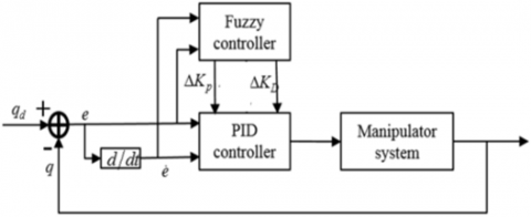
Figure 2. F-PD controller
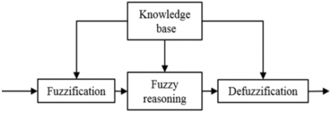
Figure 3. Fuzzy logic system
Figure 2 presents the configuration of classic F-PD, such that $q_d$ represents the standard desired input and the error $e=$ $q-q_d$ with its derivation $\dot{e}=\dot{q}-\dot{q}_d$ are selected as Fuzzy Logic inputs. The fuzzy controller's sequential coefficients $\Delta K_P$ and $\Delta K_D$ are used for the outputs of PD controller. The main steps of fuzzy logic system are shown in Figure 3. For the inputs, scaling and fuzzy rules are initially performed to convert the better product quality into the fuzzy inputs described inside the fuzzy range between -3 to 3 in this research. The results are computed using the Center of Mass defuzzification methodology (COM) and the scalable scheme of the fuzzy outputs $\Delta K_P$ and $\Delta K_D$, that are also described inside a range between -3 to 3 in this research. At fuzzification, the membership function layout will undoubtedly and immediately affect the outcome of fuzzy theory in addition to, as a response, the effectiveness of PD control.
To understand the connection between membership function and PD control performance, NMF, SMF, and ORMF are established to statistically describe the numbers of membership functions, geometry of membership functions, and overlaying rate of membership functions, respectively. For simplicity and clarity of this research, we consider the overlaying rate among the forementioned functions. NMF has seven fuzzy values. These can be described as LP, MP, SP, Z, SN, MN, LN, which indicate Large Positive, Medium Positive, Small Positive, Zero, Small Negative, Medium Negative, and Large Negative respectively. The following are the Gaussian functions that determine the appropriate membership functions for LN and LP:
$f_i\left(x, \sigma_i, \mu_i\right)=e^{\frac{-\left(x-\mu_i\right)^2}{2 \sigma_i^2}}$ (9)
where, i=1, 2, 3, …7.
Represents a Gaussian distribution function, denoted as fi. It is a probability density function used to model continuous random variables. The function depends on three parameters: x, which is the input variable; σi, representing the standard deviation and controlling the spread of the distribution; and μi, which denotes the mean or peak value of the distribution. The Gaussian function is symmetric around the mean and decreases as x moves away from the mean. A smaller σi results in a steeper curve with less variability, while a larger σileads to a wider curve with higher variability. This function finds widespread applications in various fields, including statistics, signal processing, and machine learning, due to its ability to accurately model real-world data distributions.
The Gaussian function's prediction and conventional variance are represented by σi and μi. The equivalent membership functions for other fuzzy terms are created as triangular functions:
$f_i\left(x, a_i, b_i, c_i\right)=\left\{\begin{array}{cc}0 & x \leq a_i \\ \frac{x-a_i}{b_i-a_i} & a_i \leq x \leq b_i \\ \frac{a_i-x}{c_i-b_i} & b_i \leq x \leq c_i \\ 0 & c_i \leq x\end{array}\right.$ (10)
If I=2, 3, …. 6, ai and ci are the zero points, and bi is the membership function's peak point. The deriving process is formed by the (If-Then) parallel fuzzy rules, which describe how to transfer input parameters to an output vector. The rule can be described as follows:
If x1 is A and x2 is B, then y is C.
Where x1 and x2 represent the input, y represents the result, and A, B, and C represent the fuzzy rules. The fuzzy sets for the traditional Fuzzy-PD are shown below in Tables 2 and 3.
Table 2. Fuzzy rules for $\Delta K_P$
|
|
LN |
MN |
SN |
Z |
SP |
MP |
LP |
|
LN |
LN |
LN |
LN |
MN |
MN |
Z |
Z |
|
MN |
LN |
LN |
MN |
MN |
SN |
Z |
Z |
|
SN |
MN |
MN |
SN |
SN |
Z |
SP |
SP |
|
Z |
MN |
SN |
SN |
Z |
SP |
SP |
MP |
|
SP |
SN |
SN |
Z |
SP |
SP |
MN |
MN |
|
MP |
Z |
Z |
SP |
MP |
MP |
LP |
LP |
|
LP |
Z |
Z |
SP |
MP |
LP |
LP |
LP |
Table 3. Fuzzy rules for $\Delta K_D$
|
|
LN |
MN |
SN |
Z |
SP |
MP |
LP |
|
LN |
SP |
SP |
Z |
Z |
Z |
LP |
LP |
|
MN |
SN |
SN |
SN |
SN |
Z |
LP |
LP |
|
SN |
LN |
LN |
MN |
SN |
Z |
SP |
MP |
|
Z |
LN |
MN |
MN |
SN |
Z |
SP |
MP |
|
SP |
LN |
MN |
SN |
SN |
Z |
SP |
SP |
|
MP |
MN |
SN |
SN |
SN |
Z |
SP |
SP |
|
LP |
SP |
Z |
Z |
Z |
Z |
LP |
SP |
The Mamdani fuzzification approach is chosen depending on the basis functions and fuzzy sets. Since the divining strategy for $\Delta K_P$ and $\Delta K_D$ are similar, just the procedure to find $\Delta K_P$ is described in the next section. In Eq. (4), the fuzzy output of $\Delta K_P$ is determined as follows:
$f p(x)=\sqrt{\left(f_i^E \Lambda f_j^{E C} \Lambda f_k^{\Delta K_P}\right)}$ (11)
The Eq. (11) represents a fuzzy logic function used to compute a final performance value, denoted as $f_p(x)$. This function involves the combination of three intermediate fuzzy membership values: $f_i^E, f_i^E C$, and $f_k^{\Delta K_P}$. These membership values are obtained through fuzzy logic operations, such as the AND operation (represented by the symbol $\wedge$ ), which allows the system to reason with multiple input conditions.
The interpretation of the fuzzy logic function is as follows: $f_i^E, f_i^E C$, and $f_k^{\Delta K_P}$ are fuzzy membership values representing the degree of membership of the input $x$ in three different fuzzy sets $E, E C$, and $\Delta K_P$ respectively. The function combines these memberships using the AND operation, reflecting the minimum membership value of the three sets. The result is then taken as the square root, yielding the final performance value $f_p(\mathrm{x})$.
Fuzzy logic is valuable in situations where precise mathematical relationships are challenging to define, and linguistic variables and expert knowledge are more appropriate for making decisions. The $f_p(\mathrm{x})$ function with fuzzy logic enables the integration of multiple input conditions and uncertainties, making it suitable for applications in control systems, decision-making processes, and various fields where uncertainty and vagueness are prevalent.
Where i, j, and k are integer values between 1 to 7, in which they are referring to the seven fuzzy rules. With the use of COM defuzzification technique, the fuzzy outputs can be described as follows:
$\Delta K^{f p}=\frac{\int_{x=-3}^{x=3} x \cdot f_p(x) d x}{\int_{x=-3}^{x=3} f_p(x) d x}$ (12)
The Eq. (12) is used to determine the change in kinetic energy, denoted as ΔKfp, using integration with respect to a fuzzy logic performance function fp(x). This calculation involves two definite integrals, one for the product of x and the performance function fp(x) and another for fp(x) alone, both integrated over the range from x=−3 to x=3.
The interpretation of this expression is as follows:
The numerator $\int_{x=-3}^{x=3} x \cdot f_p(x) d x$ calculates the weighted average of $x$ using the fuzzy logic performance function $f_p(x)$ as the weighting factor. It represents the contribution of different $x$ values to the overall kinetic energy. The denominator $\int_{x=-3}^{x=3} f_p(x) d x$ calculates the overall degree of membership (or the total weighting) of the fuzzy logic performance function $f_p(x)$ within the range from $x=-3$ to $x=3$.
By dividing the numerator by the denominator, the expression yields the change in kinetic energy ΔKfp based on the fuzzy logic performance function fp(x). This approach allows for the incorporation of fuzzy logic principles into the calculation of kinetic energy changes, which can be particularly useful in scenarios where precise mathematical relationships are uncertain or difficult to define, and fuzzy logic offers a more flexible and adaptable solution.
Based on the scalability procedure, the precise outputs are eventually designated as shows in Eq. (13):
$\begin{aligned} \Delta K_P=\frac{\Delta K_{\max }^P+}{2} & K_{\min }^P +k_p\left(\Delta K^{f p}-\frac{\Delta K_{\max }^{f P}+K_{\min }^{f P}}{2}\right)\end{aligned}$ (13)
Knowing that
$k_p=\frac{\Delta K_{\max }^P-K_{\min }^P}{\Delta K_{\max }^{f P}-K_{\min }^{f P}}$ which is representing as an output scaling factor.
$\Delta K_{\max }^P$ is the highest level of crisp output.
$\Delta K_{\min }^P$ is the smallest amount of crisp output.
$\Delta K_{\max }^{f p}$ is the highest level of Fuzzy output.
$\Delta K_{\min }^{f p}$ is the smallest amount of Fuzzy output.
Therefore, the usual PD controller cab be presented as follows:
$\tau_s=K_P e+K_D \dot{e}$ (14)
This controller represents a control law for a proportionalderivative (PD) controller, where $\tau_s$ is the control signal or output, $K_P$ is the proportional gain, $K_D$ is the derivative gain, $e$ is the error, and $\dot{e}$ is the derivative of the error with respect to time.
The interpretation of this control law is as follows: In a PD controller, the control signal $\tau_s$ is determined by two components. The first component, $K_P e$, is the proportional term, where the control signal is directly proportional to the error $e$ between the desired setpoint and the actual process variable. The proportional gain $K_P$ determines the sensitivity of the controller to the error, influencing how quickly the controller responds to deviations from the setpoint.
The second component, $K_D \dot{e}$, is the derivative term, where the control signal is proportional to the rate of change of the error (e). The derivative gain KD controls the damping effect of the controller and helps to stabilize the system by reducing overshoot and oscillations.
By combining the proportional and derivative terms, the PD controller provides a balance between fast response to errors (proportional term) and stability (derivative term). This control law is widely used in various control systems and applications, such as in robotics, process control, and motion control, to achieve accurate and stable control of dynamic systems.
where:
$\begin{aligned} & K_P=K_{P 0}+\Delta K_P \\ & K_D=K_{D 0}+\Delta K_D\end{aligned}$
$K_{D 0}$ and $K_{P 0}$ are represented the initial parameters chosen for $K_D$ and $K_P$ respectively.
The characteristic variables $\left(a_i, b_i, c_i, \eta_i, \sigma_i\right)$ are mostly chosen by many researchers and, therefore, set via the fuzzy inference procedure during the aforementioned Fuzzy Logic system design.
Due to the membership function is in control of converting crisp input to fuzzy input, parameters' choice $\left(a_i, b_i, c_i, \eta_i, \sigma_i\right)$ will immediately affect the overlaying rate of each two neighboring membership functions, hence the effectiveness of PD control. The membership function has a total of 19 factors that are specified as $\left(a_i, b_i, c_i, \eta_i, \sigma_i\right)$.
For $i=1,2,3, \ldots, 7$, there are two limitations that are set to facilitate the optimization technique as follows:
$c_i$ has zeros on the right side of $\mathrm{LN}$ and $\mathrm{MN}$, while $a_i$ has ones on the left side of MP and LP. Both are variables which can be changed, while the other zeros are constants.
Although only $\left(a_5, a_6, c_2, c_3\right)$ are selected as the ORMF influencing criteria under the aforementioned two conditions, the challenge of this research is to attain ORMF improvement by improving the values of $\left(a_5, a_6, c_2, c_3\right)$. Next section will explain in detail the ORMF optimization method.
The motivation behind using Back Propagation Neural Network (BPNN) in robot control lies in its ability to learn complex control policies from data and adapt to non-linear and uncertain environments. BPNN is a type of artificial neural network that utilizes supervised learning to adjust its internal parameters and optimize its performance based on training data. In robot control applications, BPNN can be trained with data generated from simulations or real-world robot interactions, allowing it to learn intricate mappings between sensory inputs and corresponding control outputs. This learning capability enables robots to handle intricate tasks and dynamically adapt to changing conditions, making them more versatile and efficient in various environments. BPNN’s ability to approximate non-linear functions allows it to model intricate robot dynamics and system behaviors more accurately, improving control precision and performance. Moreover, the trained neural network can generalize from the learned data, allowing robots to navigate complex environments, interact with objects, and perform tasks with greater autonomy and reliability. By integrating BPNN into robot control systems, robots can become more intelligent, adaptive, and capable of handling sophisticated tasks in diverse applications, ranging from industrial automation to autonomous navigation and human-robot interaction.
The choice to use a Back Propagation Neural Network (BPNN) in robotic control stems from its ability to learn and adapt complex control policies from data, making it a powerful tool in enhancing robotic capabilities. In their overall robotic control system, the researchers opted for BPNN due to its supervised learning approach, which allows it to adjust internal parameters and optimize performance based on training data. By training the BPNN with data collected from simulations or real-world robot interactions, it can learn intricate mappings between sensory inputs and corresponding control outputs. This learning capability complements the robot's control framework, enabling it to handle non-linear and uncertain environments more effectively. Integrating BPNN into their robotic control system empowers the robot to become more intelligent, versatile, and autonomous. It allows the robot to dynamically adapt to changing conditions, improve control precision, and perform intricate tasks with greater reliability. As a result, the incorporation of BPNN enhances the overall robotic control strategy, making the robot more capable and efficient in various applications, ranging from industrial automation to autonomous navigation and human-robot interaction.
As mentioned in the previous section, the variables ai and ci in Eq. (3) are the threshold parameters of each associated membership function.
Changing these variables will affect ORMF and the F-PD controller's output. The four variables $\left(a_5, a_6, c_2, c_3\right)$ are chosen as the ORMF criteria based on the two limitations described above (at the end of the last section). As a result, they will be constructed as the Neural Network with Back-Propagation's output. The input is the system's error and its derivative, which indicates the performance of a system. Figure 4 illustrates the basic principle of Neural Network with Back-Propagation, which includes three layers (input, hidden, output).
Figure 4. Back Propagation Neural Network design
In Figure 4, x={x1,...xi,...xp} represents the input, and y=y1,...yz,...yg represents the overall output. The outcome of the input layer will be as:
$O_m^{(1)}=x(m)$ (15)
The input and output hidden layer will be shown as:
$n e t_n^{(2)}(\mathrm{k})=\sum_{m=1}^2 w_{n m}^{(2)} O_m^{(1)}$ (16)
$n e t_n^{(2)} O_n^{(2)}(\mathrm{k})=f\left(n e t_n^{(2)}(k)\right)$ (17)
when n=1, 2, 3, ..., q.
The neurons number is denoted by q.
The present sample number is k.
The activating function f(x) can be represented as a sigmoid function, which is described in below:
$f(x)=\frac{e^x-e^{-x}}{e^x+e^{-x}}$ (18)
Therefore, the production layers' input and output are specified as follows:
$n e t_n^{(3)}(\mathrm{k})=\sum_{n=0}^q w_{l n}^{(3)} O_m^{(2)}(k)$ (19)
$O_l^{(3)}(\mathrm{k})=\mathrm{g}\left(n e t_l^{(3)}(k)\right)$ (20)
Knowing that
l=1,2, 3, and 4.
$\begin{aligned} & O_1^{(3)}(k)=c_2, O_2^{(3)}(k)=c_3 \\ & O_3^{(3)}(k)=a_5, O_4^{(3)}(k)=a_6\end{aligned}$
$w_{l n}^{(3)}$ denotes the weight from the hidden layer to the production layer.
g(x) is the activation function, that is described in the following formula:
$g(x)=\frac{e^x}{e^x+e^{-x}}$ (21)
The cost formula will be as follows:
$E=0.5\left(q_r-q\right)^2=0.5 e^2$ (22)
The production layer's weight parameter may be produced by coupling the gradient descent approach with an inertial component. In general, it makes the research a rapid convergence. Also, the weight parameter can be defined as:
$\Delta w_{l n}^{(3)}(k)=-\eta \frac{\partial E(k)}{\partial w_{l n}^{(3)}}+\alpha \Delta w_{l n}^{(3)}(k-1)$ (23)
where, $\frac{\partial E(k)}{\partial w_{l n}^{(3)}}=\frac{\partial E(k)}{\partial \mathrm{q}(\mathrm{k})} * \frac{\partial q(k)}{\partial O_l^{(3)}(k)} * \frac{\partial O_l^{(3)}(k)}{\partial n e t_l^{(3)}(k)} * \frac{\partial n e t_l^{(3)}(k)}{\partial w_{l n}^{(3)}}$.
The learning rate is denoted by η, while the inertia factor is denoted by α.
Eq. (16) is derived throughout the learning process to simplify $\frac{\partial E(k)}{\partial w_{l n}^{(3)}}$.
$\frac{\partial q(k)}{\partial O_l^{(3)}(k)}=\frac{q(k)-q(k-1)}{\partial O_l^{(3)}(k)-\partial O_l^{(3)}(k-1)}$ (24)
And the learning rate x can adjust for the estimate effect. When Eq. (23) is substituted from Eq. (22), the update of the production layer weight can eventually be indicated as:
$\Delta w_{l n}^{(3)}(k)=-\eta \delta_l^{(3)} O_n^{(k)}+\alpha \Delta w_{l n}^{(3)}(k-1)$ (25)
where, $\delta_l^{(3)}=e(k) \frac{\partial q(k)}{\partial o_l^{(3)}(k)} \dot{g}\left(n e t_l^{(3)}(k)\right)$
l=1, 2, 3, 4.
As a result, the update weights of hidden layer are indicated as below:
$\Delta w_{n m}^{(2)}(k)=\eta \cdot \delta_l^{(2)} \cdot O_m^{(1)}(k)+\alpha \Delta w_{l n}^{(3)}(k-1)$ (26)
$\delta_l^{(2)}=e(k) \frac{\partial q(k)}{\partial O_n^{(2)}} \dot{f}\left(n e t_n^{(2)}(k)\right)$ (27)
i=1, 2, …, q
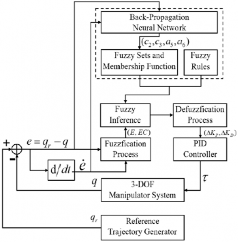
Figure 5 depicts the entire closed-loop control block and calculating procedure. Fuzzy Logic and Neural Network with Back-Propagation are fed the position error and its variation. The ORMF is improved by optimization of c2, c3, a5, a6 by Neural Network with Back-Propagation, and the fuzzy results are obtained using the Mamdani inference technique depending on improved membership function as well as the fuzzy sets. The resulting control gains $\Delta K_P, \Delta K_D$ are fed into the planned PD controller after COM defuzzification. The relevant control torques are then delivered to the robotic system.
$w_{n m}^{(2)}$ denotes the weights from the layer of input to the hidden layer, while the superscripts (1), (2), and (3) denote to the three layers respectively.
Figure 5. Control block and process
The integration of Back Propagation Neural Network (BPNN) into the Overall Robotic Motion Framework (ORMF) has led to significant improvements in the control of the 3-DOF robot arm. By employing BPNN's supervised learning approach, the ORMF was able to learn complex control policies and adapt to non-linear dynamics, enhancing the robot arm's performance and capabilities. The BPNN facilitated precise mapping between sensory inputs and control outputs, enabling more accurate and efficient control of the robot arm's movements. This improvement has profound implications for the robot's control, as it enhances its ability to navigate intricate environments, interact with objects, and perform sophisticated tasks with greater autonomy and reliability. With BPNN's dynamic adaptability and accurate modeling of the robot arm's behavior, the control system can respond more intelligently to changing conditions and uncertainties. Consequently, the robot arm becomes more versatile and efficient, making it suitable for a broader range of applications in industries like manufacturing, assembly, and automation. Ultimately, the integration of BPNN into the ORMF empowers the 3-DOF robot arm with enhanced control capabilities, leading to increased precision, robustness, and overall performance in its assigned tasks.
Simulations using MATLAB and practical trials on a 3-DOF robot arm are used to illustrate the efficiency and advantages of the suggested control technique. The robot contains three rotating joints, as shown in Figure 1. Table 4 presents the parameters of the manipulator. These include: inertia moment, length and mass.
To establish a sinusoidal reference trajectory, a 3-DOF robotic arm's end-effector is used. The following are the definitions of the reference trajectories equations.
$\left.\begin{array}{c}x=0.4 \\ y=0.02 t-0.2 \\ 0.13-0.12 \sin (16 y+3.2)\end{array}\right\} \quad 0<t \leq 20$
The position $q=\left[q_1, q_2, q_3\right]^T$ of the reference joints acquired by using inverse kinematics to the end-effector's trajectory. For modeling and tests purposes, the manipulator's starting position is set to
$q_0=\left[q_{01}, q_{02}, q_{03}\right]^T=[0.4,1,0.6]^T$
The initial Proportional-Derivative (PD) controller gains are typically determined through a process called "tuning." The goal of tuning is to find suitable values for the proportional gain (KP) and derivative gain (KD) that result in stable and satisfactory control performance for the specific robot system. There are several methods for tuning the PD controller gains. One of these methods which is used in this paper is Manual Tuning. In manual tuning, an experienced control engineer adjusts the gains iteratively based on intuition and knowledge of the system. The engineer observes the system's response to different gains and makes adjustments until the desired performance is achieved. Manual tuning is often quick and straightforward but may require expertise in control theory and system dynamics.
The initial gains of the PD controller will be as:
$K_{P O}=\left[\begin{array}{ccc}K_{P O}^1 & 0 & 0 \\ 0 & K_{P O}^2 & 0 \\ 0 & 0 & K_{P O}^3\end{array}\right]=\left[\begin{array}{lll}8 & 0 & 0 \\ 0 & 8 & 0 \\ 0 & 0 & 8\end{array}\right]$
$K_{D O}=\left[\begin{array}{ccc}K_{D O}^1 & 0 & 0 \\ 0 & K_{D O}^2 & 0 \\ 0 & 0 & K_{D O}^3\end{array}\right]=\left[\begin{array}{ccc}2 & 0 & 0 \\ 0 & 6 & 0 \\ 0 & 0 & 6\end{array}\right]$
The membership function is shown in Figure 6.
Table 4. Parameters of 3-DOF robot
|
|
Link 1 |
Link 2 |
Link 3 |
|
Inertia Moment (Kg.m2) |
0.026 |
0.022 |
0.02 |
|
Length (m) |
0.3 |
0.25 |
0.22 |
|
Mass (Kg) |
0.375 |
0.3 |
0.25 |
Figure 6. Membership function before the optimization
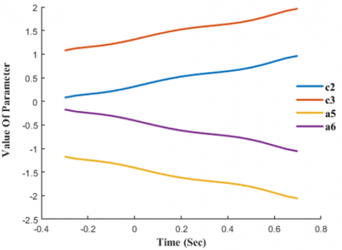
Figure 7. Parameters optimization
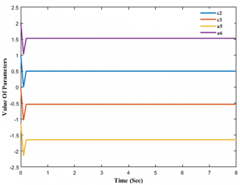
Figure 8. Joint 1 parameter value
Simulations are run in MATLAB using the 3-DOF manipulator's kinematic characteristics, the end-effector's intended reference path as well as the initial variables for PD, fuzzy logic, and neural networks with back-propagation. Figure 7 describes the improvement of the four essential factors. When the input error increases, the critical factors of the membership function will raise the ORMF under NN modification, hence increasing the F-PD controller's output and forcing the system as a whole to respond quickly.
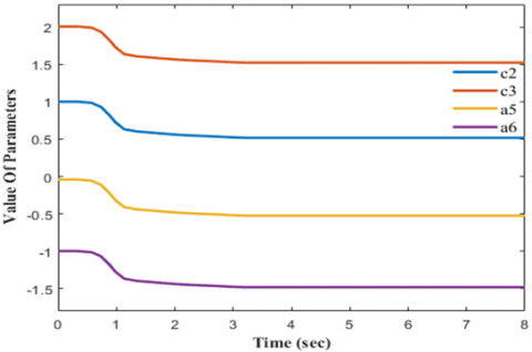
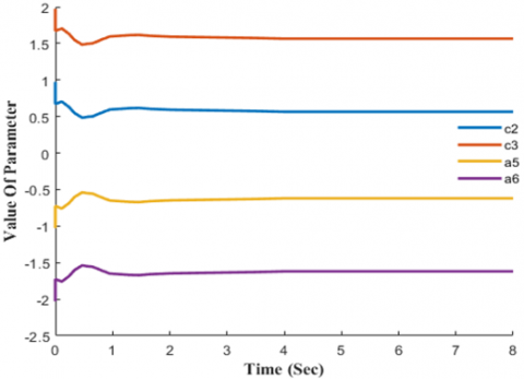
Figures 8, 9, and 10 depict the changes in each joint's critical parameters over the course of the simulation.
Figure 9. Joint 2 parameter value
Figure 10. Joint 3 parameter value
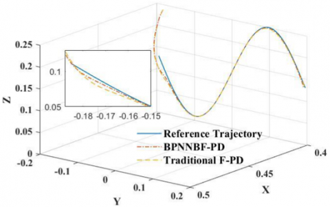
Figure 11. Trajectory tracking
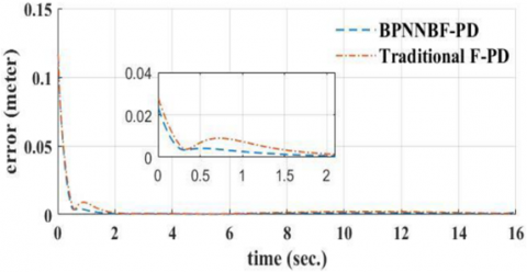
Figure 12. Trajectory tracking error
The simulation results of Fuzzy-PD based Back-Propagation Neural Network are compared with the outcomes of the classic F-PD control method to demonstrate the benefit of the proposed approach Neural Network with Back-Propagation BF PD in this article. Figures 11 and 12 demonstrate the path tracking and tracking errors for the two systems, respectively.
As seen in the previous two figures, the suggested Fuzzy-PD Based on Back-Propagation Neural Network approach is quicker, with a 25% shorter time to convergence than the typical F-PD control approach. When the robot instantly adapts to the desired trajectory, the suggested approach has an overrun of 0.006m, whereas the F-PD technique has an overshoot less than 0.01m. When compared to the conventional F-PD technique, the Fuzzy-PD Based on Back-Propagation Neural Network reduces overshoot by 49.1%.
A 49.1% reduction in overshoot and quicker response time in robot control is highly significant due to its profound impact on the robot's performance and efficiency. Overshoot reduction ensures that the robot's movements are more precise and stable, minimizing the risk of unintended collisions or errors in task execution. By reducing overshoot, the robot can reach its target position more accurately and reliably, leading to improved overall performance and safety.
Additionally, the quicker response time is crucial for time-sensitive tasks or dynamic environments. A faster response allows the robot to adapt swiftly to changing conditions, increasing its agility and responsiveness. In applications like industrial automation or autonomous navigation, quicker response times can lead to higher productivity, reduced cycle times, and better decision-making.
The combination of reduced overshoot and quicker response time significantly enhances the robot's capabilities and effectiveness, making it more reliable and efficient in accomplishing complex tasks. This approach can have a substantial impact on various industries, providing a competitive advantage and advancing the state-of-the-art in robot control technology. The comparison between PD, PI, PID, Neural Network, Fuzzy-PD, and suggested controller according to the overshoot and time response is shown in Table 5.
Table 5. Overshoot and time response values with different controllers
|
Approach Name |
Overshoot (%) |
Time Response (s) |
|
PD Control [22] |
10.2 |
3.4 |
|
PI Control [23] |
5.8 |
2.1 |
|
PID Control [24] |
3.2 |
1.8 |
|
Neural Network (NN) Control [25] |
1.5 |
1.2 |
|
Fuzzy- PD [26] |
1 |
1.8 |
|
Optimization of Fuzzy-PD Using Back-Propagation Neural Network [Suggested] |
0.6 |
1.25 |
The limitations of "Fuzzy-PD Control for a Robotics Manipulator using a Back-Propagation Neural Network" can include the following:
Fuzzy-PD based on Back-Propagation Neural Network is suggested in this research to enhance Mamdani fuzzy prediction method by continuous adjustment of membership function overlaying rate. To explain the membership function of the Fuzzy Logic model, three criteria are initially defined: NMF, SMF, and ORMF. Just the relation involving ORMF and system control efficiency is thoroughly examined. Neural Network with Back-Propagation is used in continuous learning and training to determine the ideal membership function border variables, which directly impact ORMF. Simulations using a 3-DOF robotics arm show that the suggested approach outperforms the standard F-PD technique. Overall, the integration of Fuzzy-PD based on Back-Propagation Neural Network offers a robust and adaptive control system for a 3-DOF robot arm. It enables more accurate, flexible, and efficient control, making the arm better suited for a wide range of tasks, from precise manipulations to handling uncertainties in real-world environments by reducing the overshoot with 50% and reduce the response time by 25% when compared results with standard Fuzzy -PD approach.
Our future works can include the following. These suggestions could also cover the limitation of our current research:
[1] Mandava, R.K., Vundavalli, P.R. (2015). Design of PID controllers for 3-DOF planar and spatial manipulators. In International Conference on Robotics, Automation, Control and Embedded Systems, Chennai, India, pp. 1-6. https://doi.org/10.1109/RACE.2015.7097269
[2] Liu, D., Wang, Y., Wan, X., Lai, X. (2018). Position control of a planar four-link underactuated manipulator. In 37th Chinese Control Conference, Wuhan, China, pp. 929-932. https://doi.org/10.23919/ChiCC.2018.8483418
[3] Abdul-Sadah, A.M., Raheem, K.M.H., Altufaili, M.M.S. (2022). A fuzzy logic controller for a three links robotic manipulator. In AIP Conference Proceedings, Najaf, Iraq. https://doi.org/10.1063/5.0066871
[4] Xiong, J., Liu, J. (2013). The robust step performance of PID and fuzzy logic controlled SISO systems. In Chinese Control and Decision Conference, Guiyang, China, pp. 1370-1375.
[5] Wang, J., Jordan, J.R. (1995). Neural network PID controller auto-tuning design and application. In IEEE International Conference on Fuzzy Systems, Yokohama, Japan, pp. 325-330. https://doi.org/10.1109/CCDC.2013.6561139
[6] Abbas, G., Abouchi, N., Sani, A., Condemine, C. (2011). Design and analysis of fuzzy logic based robust PID controller for PWM-based switching converter. In IEEE International Symposium of Circuits and Systems, 5(7): 777-780. https://doi.org/10.1109/ISCAS.2011.5937681
[7] Sharma, K., Palwalia, D.K. (2017). A modified PID control with adaptive fuzzy controller applied to DC motor. In International Conference on Information, Communication, Instrumentation and Control, Indore, India, pp. 1-6. https://doi.org/10.1109/ICOMICON.2017.8279151
[8] Rattan, K.S., Van Cleave, D. (2000). Design and implementation of a reduced rule fuzzy logic PID controller. In 19th International Conference of the North American Fuzzy Information Processing Society, Atlanta, GA, USA, pp. 465-469. https://doi.org/10.1109/NAFIPS.2000.877475
[9] Brehm, T., Rattan, K.S. (1994). Hybrid fuzzy logic PID controller. In IEEE 3rd International Fuzzy Systems Conference, Orlando, FL, USA, pp. 1682-1687. https://doi.org/10.1109/NAECON.1993.290839
[10] Xia, J., Xia, C. (2007). Fuzzy logic based adaptive PID control of switched reluctance motor drive. In Chinese Control Conference, Hunan, China, pp. 41-45. https://doi.org/10.1109/CHICC.2006.4347328
[11] Pereira, J., Bowles, J.B. (1994). A comparison of PID and fuzzy control of a model car. In IEEE 3rd International Fuzzy Systems Conference, Orlando, FL, USA, pp. 849-854. https://doi.org/10.1109/FUZZY.1994.343846
[12] Hirulkar, S., Damle, M., Rathee, V., Hardas, B. (2014). Design of automatic car breaking system using fuzzy logic and PID controller. In International Conference on Electronic Systems, Signal Processing and Computing Technologies, Nagpur, India, pp. 413-418. https://doi.org/10.1109/ICESC.2014.81
[13] Wen, X., Liao, Q., Wei, S., Li, R. (2009). Research and design of controller for translational meshing motor based on fuzzy logic and PID. In 2nd International Conference on Power Electronics and Intelligent Transportation System, Shenzhen, China, pp. 418-421. https://doi.org/10.1109/PEITS.2009.5406750
[14] Du, M., Wang, L. (2011). A parameter self-tuning fuzzy-PID control system for pneumatic manipulator of library robot. In International Conference on Electronics, Communications and Control, Ningbo, China, pp. 4111-4115. https://doi.org/10.1109/ICECC.2011.6067700
[15] Meza, J.L., Soto, R., Arriaga, J. (2009). An optimal fuzzy self-tuning PID controller for robot manipulators via genetic algorithm. In Eighth Mexican International Conference on Artificial Intelligence, Guanajuato, Mexico, pp. 21-26. https://doi.org/10.1109/MICAI.2009.34
[16] Siddique, M.N.H., Tokhi, M.O. (2002). GA-based neuro-fuzzy controller for flexible-link manipulator. In IEEE International Conference on Control Applications, Glasgow, UK, pp. 471-476. https://doi.org/10.1109/CCA.2002.1040231
[17] Liu, F., Gao, G., Shi, L., Lv, Y. (2017). Kinematic analysis and simulation of a 3-DOF robotic manipulator. In 3rd IEEE International Conference on Computational Intelligence and Communication Technology (CICT), Ghaziabad, India, pp. 1-5. https://doi.org/10.1109/CIACT.2017.7977291
[18] Raheem, K.M.H., Hassoon, O.O., Abdul-Sadah, A.M. (2022). Modeling 3-Degree of Freedom robotics manipulator with PID and sliding mode controller. In AIP Conference Proceedings, Najaf, Iraq. https://doi.org/10.1063/5.0066824
[19] Yu, Y., Qi, P., Althoefer, K., Lam, H.K. (2015). Lagrangian dynamics and nonlinear control of a continuum manipulator. In IEEE Conference on Robotics and Biomimetic, China, pp. 6-9. https://doi.org/10.1109/ROBIO.2015.7419052
[20] Raheem, K.M.H., Najaf, A.N. (2020). Simulation 3-DOF RRR robotic manipulator under PID controller. Journal of Engineering & Applied Sciences, 15(2): 410-414. http://doi.org/10.36478/jeasci.2020.410.414
[21] Saleh, M.H., Elassal, A.H., Khalifa, I.H. (1997). An adaptive fuzzy controller to improve system performance. In the 7th Conference on Computer and Applications, IEEE Alex. Chapter, Alexandria, Egypt.
[22] Kabir, U., Fatihu, M., Haruna, H., Shehu, G.S. (2019). Performance analysis of PID, PD and fuzzy controllers for position control of 3-DOF robot manipulator. Zaria Journal of Electrical Engineering Technology, 8(1): 12076.
[23] Joyo, M.K., Raza, Y., Ahmed, S.F., Billah, M.M., Kadir, K., Naidu, K., Yusof, Z.M. (2019). Optimized proportional-integral-derivative controller for upper limb rehabilitation robot. Electronics, 8(8): 826. https://doi.org/10.3390/electronics8080826
[24] Van Bach, N.P., Hai, Q.D., Trung, T.B. (2021). Optimization of trajectory tracking control of 3-DOF translational robot use PSO method based on inverse dynamics control for surgery application. Journal of Vibroengineering, 23(7): 1591-1601. https://doi.org/10.21595/jve.2021.21997
[25] Luan, F., Na, J., Huang, Y., Gao, G. (2019). Adaptive neural network control for robotic manipulators with guaranteed finite-time convergence. Neurocomputing, 337: 153-164. https://doi.org/10.1016/j.neucom.2019.01.063
[26] Chen, S., Yu, H., Tan, Z., Huang, J., Zhou, D., Li, H. (2022). Fuzzy proportional-derivative based robot arm control for object transfer. In 2022 International Conference on Energy Utilization and Automation (ICEUA 2022), p. 012036. https://doi.org/10.1088/1742-6596/2254/1/012036