Israa A. Ibrahim![]() | Wafaa M. Taha
| Wafaa M. Taha![]() | Mizal Alobaidi
| Mizal Alobaidi![]() | Ali F. Jameel*
| Ali F. Jameel*![]() | Eihab Bashier
| Eihab Bashier![]() | Nawal H. Alshirawi
| Nawal H. Alshirawi![]()
© 2024 The authors. This article is published by IIETA and is licensed under the CC BY 4.0 license (http://creativecommons.org/licenses/by/4.0/).
OPEN ACCESS
The fundamental purpose of this investigation is to make use of an analytical approach in order to solve and assess initial boundary value problems that are in the form of fractional partial differential equations (FPDEs). Intricate scientific phenomena that are marked by hereditary characteristics that are passed down from one generation to the next can be better understood with the help of the FPDEs, which are extremely useful instruments. In particular, when working with non-linear equations, it can be difficult to obtain analytical solutions that are either exact or approximate for these equations. In order to address these obstacles, the homogeneous balancing method (HBM) is being investigated in great detail and expanded in an innovative way in order to solve nonlinear physical problems that include FPDEs. HBM is renowned for its capacity for solving both linear and nonlinear fractional models, employing a direct approach that utilises a closed-form solution. The present study introduces an expanded version of the HBM that integrates the ideas of fractional calculus, specifically focusing on fractional derivative techniques. The approach is illustrated by analytically solving and examining two types of nonlinear FPDEs: the space-time fractional-coupled Burger's equation and the conformable fractional version of the Gerdjikov-Lvanov equations (GL), which encompass hyperbolic, trigonometric, and rational solutions. The efficiency of the extended form of the HBM is demonstrated by analyzing and comparing the acquired results with those reported in the literature. HBM would make a significant contribution towards overcoming the obstacles of existing methods, such that the proposed method will help us simplify the complexity of the nonlocal derivative when solving FPDEs. Overall, this work presents a feasible and efficient analytical approach for solving nonlinear FPDE using an extension form of the HD method with result analysis.
fractional differential equation, boundary value problems, homogeneous balance method (HBM), space- time fractional coupled Burger’s equation, Gerdjikov-Lvanov equations (GL)
Indeed, fractional-order models can offer more precise and adaptable representations of systems that exhibit long-term memory effects [1]. Fractional calculus provides a potent mathematical technique for capturing such effects by permitting the use of derivatives and integrals with non-integer orders. Nevertheless, it is crucial to acknowledge that the utilisation of fractional calculus is not universally essential or suitable, and conventional integer-order models can still be efficacious for numerous practical applications [2].
Moreover, although fractional calculus has a lengthy historical background that dates back to the 17th century, its application in engineering and research has experienced significant growth in recent years. This can be attributed to advancements in computing capabilities and the demand for more advanced modelling methods [3]. Fractional calculus remains a nascent and dynamic discipline, characterised by continuous investigation and advancement of novel techniques and practical uses [4, 5]. To summarize, fractional calculus is a potent mathematical technique used to represent systems that exhibit long-term memory effects. However, it is not universally necessary or suitable for all applications. Traditional calculus remains applicable in several real-world situations, while the utilisation of fractional calculus necessitates meticulous evaluation and specialized knowledge. This observation emphasises the significance of resolving intricate models within the realm of fractional calculus theory. To completely comprehend the physical and technical features of the problem, it is crucial to not only accurately model complicated real-world problems using this theory, but also to obtain solutions to these models [6]. Recently, there have been significant advancements in applied sciences and engineering in this field. These include areas such as biological processes, control theory, electrical networks, groundwater flow and Geo-Hydrology, viscoelasticity, finance systems, wave propagation, plasma physics and fusion, rheology, chaotic processes, and fluid mechanics, among others [7-12].
By solving these models, researchers can gain a better understanding of the system's behaviour, which in turn allows them to make more accurate predictions and develop more effective remedies. Nevertheless, owing to the intricate dynamics at play, solving these models can be no easy feat. Researchers have made efforts to create analytical methods and algorithms that can solve these models, and they are still working on making these methods better. Engineering, physics, economics, and many more disciplines rely on precise answers to complicated models to advance their respective professions [13].
The popularity and importance of the homogeneous balancing approach in finding exact solutions for travelling waves [13]. This algebraic technique was first proposed by Fan and has since been developed by other researchers [14-19]. The method involves finding a nonlinear transformation that can be used to obtain an exact solution to the problem at hand [14, 15].
Fractional calculus is a branch of calculus that generalizes the traditional calculus operators of differentiation and integration to non-integer orders. In other words, fractional calculus deals with the concept of fractional or non-integer order differentiation and integration. This section presents some the basic concepts and definitions linked with fractional calculus theory, which will help us comprehend the study in the next sections.
Definition 1: Let there be a continuous function f such that $f: R \rightarrow R$, $t \rightarrow f(t)$ then it is Riemann Liouville derivatives of fractional order α is expressed below [20]:
$\begin{gathered}D_c^\alpha=\frac{1}{\Gamma(1-\alpha)} \frac{d}{d x} \int_c^x \frac{f(t)}{(x-t)^{\alpha-m+1}} d t \\ 0<\alpha<1\end{gathered}$ (1)
$\begin{gathered}D_c^\alpha=\frac{1}{\Gamma(m-\alpha)} \frac{d^m}{d x^m} \int_c^x \frac{f(t)}{(x-t)^{\alpha-m+1}} d t \\ 0<\alpha<1\end{gathered}$ (2)
From Eq. (1) and Eq. (2) we get
$\begin{gathered}D^\alpha t^m=\frac{\Gamma(1+m)}{\Gamma(1+m-\alpha)} t^{m-\alpha}, m>-1, \\ 0<\alpha<1\end{gathered}$ (3)
Some Liouville derivative:
If $f: R \rightarrow R$ continuous function, then its fractional derivative in the form of integral with respect to $(d x)^\alpha$:
$D_x^\alpha f(x)=\frac{1}{\Gamma(\alpha)} \int_0^x(x-\tau)^{\alpha-1} f(\tau) d(\tau)=\frac{1}{\Gamma(1-\alpha)} \frac{d}{d x} \int_0^x f(\tau)(d(\tau))^\alpha, 0<\alpha<1$ (4)
Fractional derivative for the linear combination of the functions $f(x)$ and $g(x)$ and the constants $a$ and $b$ is define as:
$D_x^\alpha(a f(x)+b g(x))=a D_x^\alpha(f(x))+b D_x^\alpha(g(x))$ (5)
For $f(x)=x^k$, the fractional derivative is:
$D_x^\alpha\left((x)^k\right)=\frac{\Gamma(1+k)}{\Gamma(1+k-\alpha)}(x)^{k-\alpha}$ (6)
Definition 2: Let $f:[0, \infty) \rightarrow R$ be a function. Then its fractional conformable derivative which is $\alpha$ th order is [21]:
$T_\alpha f(x)=\lim _{\varepsilon \rightarrow 0} \frac{f\left(x+\varepsilon x^{1-\alpha}\right)-f(x)}{\varepsilon}$, (7)
where, $\alpha \in(0,1)$ and it hold for all $x>0$.
If the function $f$ is $\alpha$-differentiable in $(0,1)$ for $l>0$ and further;
If the function $f$ is $\alpha$-differentiable in $(0,1)$ for $l>0$ and further $\lim _{x \rightarrow 0^{+}} f^{(n)}(x)$ exists, then the conformable derivative at 0 is defined:
$f^n(0)=\lim _{x \rightarrow 0^{+}} f^{(n)}(x)$ (8)
Also, the conformable integral of function $f$ is defined as:
$I_\alpha^l f(x)=\int_l^x \frac{f(t)}{t^{1-\alpha}} d t, l \geq 0$ and $\alpha \in(0,1]$ (9)
Definition 3: Let $f:[0, \infty) \rightarrow R$ be a function. Then its fractional conformable derivative which is $\alpha$ th order is [21]:
$D^\alpha f(x)=\lim _{\xi \rightarrow 0} \frac{f\left(x+\xi x^{1-\alpha}\right)-f(x)}{\xi}$, (10)
where, $\alpha \in(0,1)$ and it holds for all $x>0$. If the function $f$ is $\alpha$-differentiable in $(0,1)$ for $l>0$ and further $\lim _{x \rightarrow 0^{+}} f^n(x)$ exists, then the conformable derivative at 0 is defined as $f^n(0)=\lim _{x \rightarrow 0^{+}} f^n(x)$.
Theorem 1: Suppose the functions $u$ and $v$ are $\alpha$-differentiable at any point $x>0$ for $\alpha \in(0,1]$. Then we have the following properties [21]:
Consider a nonlinear conformable fractional equation to explain the fundamental concept behind our approach.
$F\left(u, u_x, u_t, D_t^\alpha u, D_x^\alpha u, D_{t t}^{2 \alpha} u, D_{x x}^{2 \alpha} u, \ldots\right), 0<\alpha<1$ (11)
where, F represents any polynomial of a function and its partial fractional derivatives. The suggested method consists of the following phases:
Step 1: Assuming the transformation
$u(x, t)=U(r), r=k \frac{x^\alpha}{\alpha}+c \frac{t^\alpha}{\alpha}$ (12)
where, k and c are unknown nonzero constants. The nonlinear FPDE in Eq. (11) was transformed into the non-linear ordinary differential equation.
$H\left(U, \mathrm{U}^{\prime}, \mathrm{U}^{\prime \prime}, U^{\prime \prime \prime}, \ldots\right)=0$ (13)
Here, $H$ is a function of $U(r)$, and the prime indicates its derivatives with respect to $r$.
Step 2: Suppose that Eq. (13) has a solution of the form.
$U(r)=\sum_{i=0}^n a_i \varphi^i$ (14)
where, $a_i(i=0,1,2, \ldots n)$ are constant to be computed later, n is a positive integer chosen by balancing the highest order derivatives term with the nonlinear term in Eq. (13).
Step 3: Eq. (14) may be substituted for (13), yielding the algebraic system of equations. This system's solution can be obtained by using Maple and the answers to Eq. (13) are all precise solutions to Eq. (11).
In this section, two nonlinear FPDE test problems are considered to illustrate the performance of the proposed HB method.
4.1 The space–Time fractional–Coupled burgers equation
Consider the space –time fractional coupled Burger equation [22]:
$D_t^\alpha u-D_x^{2 \alpha} u+2 u D_x^\alpha u+\lambda D_x^\alpha(u v)=0, t>0,0<\alpha \leq 1$ (15)
$D_t^\alpha v-D_x^{2 \alpha} v+2 v D_x^\alpha v+\mu D_x^\alpha(u v)=0, t>0,0<\alpha \leq 1$ (16)
We employ the newly defined transformation to study precise wave solutions to Eqs. (15)-(16):
$u(x, t)=U(r), v(x, t)=V(r), r=\frac{x^\alpha}{\Gamma(1+\alpha)}+\frac{c t^\alpha}{\Gamma(1+\alpha)}$ (17)
Eqs. (5)-(6) can be changed into an ODE system:
$c U^{\prime}-U^{\prime \prime}+2 U U^{\prime}+\lambda(U V)^{\prime}=0$ (18)
$c V^{\prime}-V^{\prime \prime}+2 V V^{\prime}+\mu(U V)^{\prime}=0$ (19)
Balancing number $n=1$ can be obtained by balancing $U^{\prime \prime}$ and $U U^{\prime}$ and $m=1$ can be obtained by $V^{\prime \prime}$ and $V V^{\prime}$ in Eqs. (18)-(19). The solutions can be expressed as follow:
$U=a_0+a_1 \varphi, V=b_0+b_1 \varphi$ (20)
where, $a_0$, $a_1$, $b_0$, $b_1$ are unknown constant. We are subsuming Eq. (17) into Eq. (19) along with Eq. (20) to collect all the coefficient with the same power of $(\varphi)^i$ and equate to zero and we solving the system of algebraic equation by using the Maple for obtained the following result.
Case 1: $a_0=-\frac{\lambda-1}{\lambda \mu-1}, a_1=\frac{-\lambda+1}{\mu \lambda-1}, b_0=\frac{-\mu+1}{\mu \lambda-1}, b_1=-\frac{-\mu+1}{\mu \lambda-1}, c=1$
$u_1=\frac{3}{2}\left(\frac{-\lambda+1}{u \lambda-1}\right)-\frac{1}{2}\left(\frac{-\lambda+1}{u \lambda-1}\right) \tanh \left(\frac{r}{2}\right)$ (21)
$v_1=\frac{1}{2}\left(\frac{-\mu+1}{\mu \lambda-1}\right)+\left(\frac{-\mu+1}{\mu \lambda-1}\right) \tanh \left(\frac{r}{2}\right)$ (22)
Case 2: $a_0=0, a_1=-\frac{-\lambda+1}{\mu \lambda-1}, b_0=0, b_1=-\frac{-\mu+1}{\mu \lambda-1}, c=-1$
$u_2=-\frac{1}{2}\left(\frac{-\lambda+1}{\mu \lambda-1}\right)-\frac{1}{2}\left(\frac{-\lambda+1}{\mu \lambda-1}\right) \tanh \left(\frac{r}{2}\right)$ (23)
$v_2=-\frac{1}{2}\left(\frac{-\mu+1}{\mu \lambda-1}\right)-\frac{1}{2}\left(\frac{-\mu+1}{\mu \lambda-1}\right) \tanh \left(\frac{r}{2}\right)$ (24)
Case 3: $a_0=0, a_1=0, b_0=-1, b_1=1, c=1$
$v_3=-\frac{1}{2}-\frac{1}{2} \tanh \left(\frac{r}{2}\right)$ (25)
Case 4: $a_0=a_1=0, b_0=0, b_1=1, c=1$
$v_4=\frac{1}{2}-\frac{1}{2} \tanh \left(\frac{r}{2}\right)$ (26)
Case 5: $a_0=-1, a_1=1, b_0=b_1=0, c=1$
$u_5=-\frac{1}{2}-\frac{1}{2} \tanh \left(\frac{r}{2}\right)$ (27)
Case 6: $a_0=0, a_1=1, b_0=b_1=0, c=-1$
$u_6=\frac{1}{2}-\frac{1}{2} \tanh \left(\frac{r}{2}\right)$ (28)
Next, we compare between the exact solution of Eq. (23) solved by our methods with exact solution of Eqs. (4)-(5) by $\left(\frac{G}{G^{\prime}}\right)$-expansion method we obtained the same solution under special value of $p=q=2 \sigma=1, \mu=0, C_1=0, C_2=1, \eta=\frac{-1}{4}, p_0=q_0=\frac{-1}{2}$ as shown in Table 1.
Table 1. Comparison between exact solution of proposed method with $\left(\frac{G}{G^{\prime}}\right)$-expansion method [23]
|
$\left(\frac{G}{G^{\prime}}\right)$-Expansion Method |
Proposed Method |
|
If $p=q=2 \sigma=1, \mu=0, C_1=0,$ $C_2=1, \eta=\frac{-1}{4}, p_0=q_0=\frac{-1}{2}$ then Eqs. (4)-(5) became $u=-\frac{1}{2}-\frac{1}{2} \tanh \left(\frac{\xi}{2}\right)$ |
Eqs. (25)-(27) are $v_3=-\frac{1}{2}-\frac{1}{2} \tanh \left(\frac{r}{2}\right)$ $u_5=-\frac{1}{2}-\frac{1}{2} \tanh \left(\frac{r}{2}\right)$ |
4.2 The conformable fractional form GL equation
Consider the conformable fractional form GL equation [24]:
$D_t^\alpha u-2 k D_x^\alpha u-\beta u D_x^\alpha u-\chi D_x^\alpha u D_x^{2 \alpha} u-\mu D_{t x x}^{3 \alpha} u-\gamma D_{x x x}^{3 \alpha} u=0, t>0,0<\alpha \leq 1$ (29)
The investigation of real constants and consideration of fractional transformation.
$U(x, t)=u(\xi), \xi=\frac{x^\alpha}{\alpha}-\lambda \frac{t^\alpha}{\alpha}$ (30)
where, $\lambda$ is a parameter which will be determined later.
Substituting Eq. (30) in Eq. (29) and integrating we get:
$(2 k-1) U+\mu \lambda U^{\prime \prime}-\frac{\beta}{2} U^2+\frac{(\gamma-\chi)}{2}\left(U^{\prime}\right)^2-\gamma U U^{\prime}=0$ (31)
Balancing the highest order derivative and nonlinear we obtained:
$U(x, t)=a_0+a_1 \varphi+a_2 \varphi^2$ (32)
substituting the Eq. (32) in Eq. (29) with derivatives of Eq. (32) then as a result we get the system of algebraic equation by equating the coefficients to zero and solving the system of equation, we get:
Case 1: $a_0=0, a_1=-a_2, a_2=a_2, \beta=\frac{-1}{2}\left(\frac{48 k \mu+\chi a_2(\mu-1)}{\mu \lambda-1}\right), \lambda=-\frac{-2 k}{\mu-1}, \gamma=\frac{-1}{2} \chi$
$u_1=\frac{-1}{4}\left(a_2 \operatorname{sech}^2 \frac{\xi}{2}\right)-\frac{1}{2}\left(a_2\right) \tanh \left(\frac{\xi}{2}\right)$ (33)
Case 2: $a_0=\frac{-4 k \mu}{\chi \mu+\chi}, a_1=\frac{48 k \mu^2}{\chi \mu^2-\chi}, a_2=\frac{-48 k \mu^2}{\chi \mu^2-\chi}, \beta=\frac{\chi \mu}{\mu+1}, \lambda=\frac{-4 k \mu-2 k}{\mu^2+2 \mu+1}, \gamma=\frac{-1}{2} \chi$
$u_2=\frac{-4 k \mu}{\chi \mu+\chi}+\frac{12 k \mu^2}{\chi \mu^2-\chi}\left(3-\tanh ^2\left(\frac{\xi}{2}\right)\right)$ (34)
Case 3: $a_0=\frac{12 k \mu}{\chi \mu-\chi}, a_1=\frac{-12 k \mu}{\chi \mu-\chi}, a_2=0, \beta=\frac{1}{2} \chi, \lambda=\frac{-2 k}{\mu-1}, \gamma=\frac{-1}{3} \chi$
$u_3=\frac{6 k \mu}{\chi \mu-\chi}+\frac{6 k \mu}{\chi \mu-\chi} \tanh \left(\frac{\xi}{2}\right)$ (35)
Case 4: $a_0=0, a_1=\frac{12 k \mu}{\chi \mu-\chi}, a_2=0, \beta=\frac{1}{2} \chi, \lambda=\frac{-2 k}{\mu-1}, \gamma=\frac{1}{3} \chi$
$u_4=\frac{6 k \mu}{\chi \mu-\chi}-\frac{6 k \mu}{\chi \mu-\chi} \tanh \left(\frac{\xi}{2}\right)$ (36)
$a_1=-a_2, a_2=a_2,$
$\beta=\frac{-1}{24} \frac{24 a_2^2 \chi^2 \mu+36 a_2^2 \chi^2 \mu-1152 a_2 \chi k \mu^2}{a_2\left(a_2 \chi \mu^2+a_2 \chi \mu-48 k \mu^2\right)}$
Case 5: $a_0=\frac{1}{24} \frac{a_2 \chi \mu+3 a_2 \chi-48 k \mu+A}{\chi},$
$\lambda=\frac{-1}{288} \frac{\left(6 a_2^2 \chi^2 \mu^2+36 a_2^2 \chi^2 \mu-576 a_2 \chi k \mu^2+12 A a_2 \chi \mu+54 a_2^2 \chi^2-1728 a_2 \chi k \mu+1382 k^2 \mu^2+36 A a_2 \chi\right)}{a_2 \chi \mu^2+a_2 \chi \mu-48 k \mu^2+A \mu+2 a_2 \chi}$,
$\gamma=\frac{1}{2} \chi$
$u_5=\frac{1}{24} \frac{a_2 \chi \mu+3 a_2 \chi-48 k \mu+A}{\chi}-\frac{1}{2} a_2-\frac{3}{2} a_2 \tanh \left(\frac{\xi}{2}\right)+ \frac{a_2}{4} \tanh ^2\left(\frac{\xi}{2}\right),$ (37)
where,
$A=\sqrt{a_2^2 \chi^2 \mu^2+6 a_2^2 \chi^2 \mu-96 a_2 \chi k \mu^2+9 a_2^2 \chi^2+96 a_2 \chi \mathrm{k} \mu+2304 k^2 \mu^2}$
Now, we will comparison between the exact solution of Eqs. (35)-(36) solved by our methods under the value $\mu=\frac{1}{2}, k=1$ with exact solution of Eqs. (20)-(22) by $\left(\frac{G}{G^{\prime}}\right)$-expansion method under the special value of $\mu=\frac{1}{2}, k=3$ we obtained the same solution shown in Table 2.
Table 2. Comparison between exact solution of HB method with $\left(\frac{G}{G^{\prime}}\right)$-expansion method [25]
|
$\left(\frac{G}{G^{\prime}}\right)$-Expansion Method |
Proposed Method |
|
If $\mu=\frac{1}{2}, k=3$ then $u_4=\frac{6}{\theta}+\frac{6}{\theta} \tanh \left(\frac{\eta}{2}\right)$ $u_5=\frac{6}{\theta}-\frac{6}{\theta} \tanh \left(\frac{\eta}{2}\right)$ |
If $\mu=\frac{1}{2}, k=-1$ then $u_3=\frac{6}{\chi}+\frac{6}{\chi} \tanh \left(\frac{\xi}{2}\right)$ $u_4=\frac{6}{\chi}-\frac{6}{\chi} \tanh \left(\frac{\xi}{2}\right)$ |
The stability of soliton solutions, as well as the Hamiltonian system characteristics is addressed in this section. The momentum of the Hamiltonian system (HSM) is given by the reference [26]:
$Q=\frac{1}{2} \int_{a_1}^{a_2} u^2 d \xi$ (38)
where, $u$ is the independent variable $a_1$, $a_2$ are arbitrary constant. The stability for the attained solutions depends on the HBM when satisfying the following condition $\frac{\partial Q}{\partial c}>0$, where $c$ is the speed of waves.
The generated solutions meet the stability requirement for the chosen parameter values. For instance, the solutions to the coupled burger equation in Eq. (26) are 0.248684 and Eq. (28) are .0.24868. Also, we obtained the result of the GL equation of Eq. (33) are 0.0016 and Eq. (36) are 35.753 meet the stability condition for the specified parameter values. Hence, for the various values of the parameters in the provided range, the soliton solutions of the other families likewise meet the condition Eq. (38), which has been illustrated graphically in the next section.
The efficient homogeneous approach is utilized to solve the space-time fractional-coupled Burger’s equation and the conformable fractional-form GL equation to get the soliton solution. The major focus of this effort is to develop novel and more general solutions for fractional order at various parameter values. Several different types of solutions have been produced in the literature by utilizing various strategies, such as trigonometric, hyperbolic, and rational kinds of solitary wave solutions by employing the HB method. Compared to previous results, we found that our approach is new and more comprehensive. Contour graphs are a new simulation of 3D graphs that provide more detailed information about the physical qualities of the exact solution. The physical behaviour of Eq. (11) is summarized and illustrated in Figures 1-8.
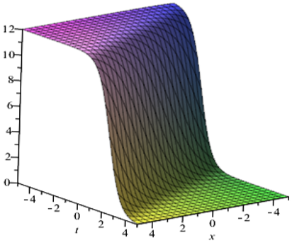
Figure 1. Solitary wave 3D graphics of Eq. (21) for $k=0.5, \alpha=1, \mu=0.2, x=-10, \ldots, 10$ and $t=-10, \ldots, 10$
Figure 2. Plot of Eq. (23) for $c=2$, $x \in[-10,10]$, $t \in[-10,10]$, contours=3 and Filledregion=true
Figure 3. The solitary wave 3D graphics of Eq. (26) for $\alpha=1, x=-10, \ldots, 10$ and $t=-10, \ldots, 10$
Figure 4. Graphics of Eq. (28) for $c=2, \alpha=1, x=-5, \ldots, 5$ and $t=-5, \ldots, 5$. Contour =3, filled region=true
Figure 5. The solitary wave 3D graphics of Eq. (35) for $\mu=0.5, k=-1, \lambda=2, x=-10, \ldots, 10 \text { and } t=-10, \ldots, 10$
Figure 6. Contour plot of Eq. (33) for $\mu=0.5, k=-1, \lambda=2, x=-5, \ldots, 5 \text { and } t=-5, \ldots, 5$. Contour=3, filledregion=true
The type wave is described from the solution $u_1(x, t)$ demonstrated in Figure 1 for choosing the parameter value for k=0.5, α=1, μ=0.2 with x=-10, …, 10 and t=-10, …, 10. Figure 2 shows the stability of the dark solitary wave solution for c=2 , x=-10,…, 10, $t \in[-10,10]$ contours=3 Filledregion=true of $u_2(x, t)$ in the interval [-5,5]. Figure 3 represents 3D of the solitary wave solution of $v_4(x, t)$ at distinct values of parameters α=1, $x \in[-10,10]$ and $t \in [-10,10]$. Figure 4 shows graphics stability of $u_6(x, t)$ for c=2, α=1, x=-5, …, 5 and t=-5, …,5. Contour =3, filled region=true in the interval [-5,5]. Figure 5 shows the wave structure solution for different values of $u_3(x, t)$ for μ=0.5, k=-1, λ=2, x=-10, …, 10 and t=-10, …,10 of Eq. (35). Stability of the bright solitary wave solution of $u_1(x, t)$ in Eq. (33) for μ=0.5, k=-1, λ=2, x=-5, …, 5 and t=-5, …,5. Contour=3, filled region=true is illustrated in Figure 6. Figure 7 presents the solitary wave 3D graphics of Eq. (36) for μ=0.5, k=-1, λ=2, x=-10, …, 10 and t=10, …,10 of $u_4(x, t)$. Figure 8 shows the stability contour plot of $u_4(x, t)$ in Eq. (36) for μ=0.5, k=-1, λ=2, x=-5,…, 5 and t=-5, …, 5. Contour=3, filled region=true.
Figure 7. The solitary wave 3D graphics of Eq. (36) for $\mu=$ $0.5, k=-1, \lambda=2, x=-10, \ldots, 10$ and $t=10, \ldots, 10$
Figure 8. Contour plot of Eq. (36) for $\mu=0.5, k=-1, \lambda=$ $2, x=-5, \ldots, 5$ and $t=-5, \ldots, 5$. Contour=3, Filledregion=true
FPDEs have grown in popularity among scholars and practitioners due to their capacity to represent and explain complicated phenomena such as boundary value problems. However, the existing analytic method is incapable of managing the computing work of solutions. Therefore, the present work focused on analyzing and formulating an analytical method, called HB, for solving some FPDEs. The HBM has the ability to obtain close form solutions with less computational work. A homogeneous balancing approach was used to effectively investigate the space-time fractional-coupled Burger’s equation. The conformable fractional form GL equation was used as a case study to demonstrate the accuracy of the HBM in solving nonlinear cases by Transforming the given FPDE into a nonlinear ordinary differential equation using the $\alpha$-dereivative operator. Moreover, the method is found to provide many distinct and accurate soliton solutions and we have tested their stability using Hamiltonian system properties. The fact that we have not observed any breaks or discontinuities in the plotted solutions is a good indication of their stability. It's also worthy to notice that reducing the value of the order of fractional derivative causes the wave to move further from the center. This suggests that the fractional derivative plays an important role in determining the behavior of the soliton solutions. The study has contributed to the field of mathematics by theoretically forming the constructed method and establishing close-from solutions with less computing work. Therefore, the developed HBM can deal with nonlinear FPDEs. Overall, this focus is in finding and analyzing soliton solutions for a particular nonlinear partial differential equation. Solitons are special solutions that have the property of maintaining their shape and velocity as they propagate through a medium. They have important applications in fields such as optics, fluid dynamics, and plasma physics. Among the examples in the experimental part of the study, the HBM version that applied in this work of HBM of several interesting FPDEs, have been created in the study to provide new reliable close from solution of the above applications which would contribute in assisting researchers to handle potential nonlinear cases with respect to these important equations.
[1] Machado, J.T., Galhano, A.M., Trujillo, J.J. (2014). On development of fractional calculus during the last fifty years. Scientometrics, 98: 577-582. https://doi.org/10.1007/s11192-013-1032-6
[2] Failla, G., Zingales, M. (2020). Advanced materials modelling via fractional calculus: challenges and perspectives. Philosophical Transactions of the Royal Society A, 378(2172): 20200050. https://doi.org/10.1098/rsta.2020.0050
[3] Jain, S., Agarwal, P. (2017). On new applications of fractional calculus. Boletim da Sociedade Paranaense de Matemática, 37(3): 113-118. https://doi.org/10.5269/bspm.v37i3.18626
[4] Bonyah, E., Atangana, A., Chand, M. (2019). Analysis of 3D IS-LM macroeconomic system model within the scope of fractional calculus. Chaos, Solitons & Fractals: X, 2: 100007. https://doi.org/10.1016/j.csfx.2019.100007
[5] Picozzi, S., West, B.J. (2002). Fractional Langevin model of memory in financial markets. Physical Review E, 66(4): 046118. https://doi.org/10.1103/PhysRevE.66.046118
[6] Jawad Hashim, D., Anakira, N.R., Fareed Jameel, A., Alomari, A.K., Zureigat, H., Alomari, M.W., Ying, T.Y. (2022). New series approach implementation for solving fuzzy fractional two-point boundary value problems applications. Mathematical Problems in Engineering, 2022: 7666571. https://doi.org/10.1155/2022/7666571
[7] Atangana, A. (2017). Fractal-fractional differentiation and integration: connecting fractal calculus and fractional calculus to predict complex system. Chaos, Solitons & Fractals, 102: 396-406. https://doi.org/10.1016/j.chaos.2017.04.027
[8] Atangana, A., Qureshi, S. (2019). Modeling attractors of chaotic dynamical systems with fractal–fractional operators. Chaos, Solitons & Fractals, 123: 320-337. https://doi.org/10.1016/j.chaos.2019.04.020
[9] Karaagac, B. (2018). Analysis of the cable equation with non-local and non-singular kernel fractional derivative. The European Physical Journal Plus, 133: 1-9. https://doi.org/10.1140/epjp/i2018-11916-1
[10] Karaagac, B. (2019). A study on fractional Klein Gordon equation with non-local and non-singular kernel. Chaos, Solitons & Fractals, 126: 218-229. https://doi.org/10.1016/j.chaos.2019.06.010
[11] Karaagac, B. (2019). Two step Adams Bashforth method for time fractional Tricomi equation with non-local and non-singular Kernel. Chaos, Solitons & Fractals, 128: 234-241. https://doi.org/10.1016/j.chaos.2019.08.007
[12] Podlubny, I. (1998). Fractional Differential Equations: An Introduction to Fractional Derivatives, Fractional Differential Equations, to Methods of Their Solution and Some of Their Applications. Elsevier. https://doi.org/10.1016/S0076-5392(99)X8001-5
[13] Choi, J.H., Kim, H., Sakthivel, R. (2014). Exact solution of the Wick-type stochastic fractional coupled KdV equations. Journal of Mathematical Chemistry, 52: 2482-2493. https://doi.org/10.1007/s10910-014-0406-1
[14] Fan, E. (2000). Two new applications of the homogeneous balance method. Physics Letters A, 265(5-6): 353-357. https://doi.org/10.1016/S0375-9601(00)00010-4
[15] Elwakil, S.A., El-Labany, S.K., Zahran, M.A., Sabry, R. (2003). Exact travelling wave solutions for the generalized shallow water wave equation. Chaos, Solitons & Fractals, 17(1): 121-126. https://doi.org/10.1016/S0960-0779(02)00414-9
[16] Elwakil, S.A., El-Labany, S.K., Zahran, M.A., Sabry, R. (2004). New exact solutions for a generalized variable coefficients 2D KdV equation. Chaos, Solitons & Fractals, 19(5): 1083-1086. https://doi.org/10.1016/S0960-0779(03)00276-5
[17] El-Wakil, S.A., Abulwafa, E.M., Elhanbaly, A., Abdou, M.A. (2007). The extended homogeneous balance method and its applications for a class of nonlinear evolution equations. Chaos, Solitons & Fractals, 33(5): 1512-1522. https://doi.org/10.1016/j.chaos.2006.03.010
[18] Khalfallah, M. (2009). New exact traveling wave solutions of the (3+1) dimensional Kadomtsev–Petviashvili (KP) equation. Communications in Nonlinear Science and Numerical Simulation, 14(4): 1169-1175. https://doi.org/10.1016/j.cnsns.2007.11.010
[19] Zhao, X., Wang, L., Sun, W. (2006). The repeated homogeneous balance method and its applications to nonlinear partial differential equations. Chaos, Solitons & Fractals, 28(2): 448-453. https://doi.org/10.1016/j.chaos.2005.06.001
[20] Antonova, M., Biswas, A. (2009). Adiabatic parameter dynamics of perturbed solitary waves. Communications in Nonlinear Science and Numerical Simulation, 14(3): 734-748. https://doi.org/10.1016/j.cnsns.2007.12.004
[21] Ma, H., Deng, A., Wang, Y. (2011). Exact solution of a KdV equation with variable coefficients. Computers & Mathematics with Applications, 61(8): 2278-2280. https://doi.org/10.1016/j.camwa.2010.09.048
[22] Mohyud-Din, S.T., Bibi, S. (2018). Exact solutions for nonlinear fractional differential equations using ($\frac{G^{\prime}}{G^2}$)-expansion method. Alexandria Engineering Journal, 57(2): 1003-1008. https://doi.org/10.1016/j.aej.2017.01.035
[23] Khatun, M.A., Arefin, M.A., Uddin, M.H., İnç, M., Akbar, M.A. (2022). An analytical approach to the solution of fractional-coupled modified equal width and fractional-coupled Burgers equations. Journal of Ocean Engineering and Science. https://doi.org/10.1016/j.joes.2022.03.016
[24] Ghanbari, B., Baleanu, D. (2020). New optical solutions of the fractional Gerdjikov-Ivanov equation with conformable derivative. Frontiers in Physics, 8: 167. https://doi.org/10.3389/fphy.2020.00167
[25] Rani, A., Zulfiqar, A., Ahmad, J., Hassan, Q.M.U. (2021). New soliton wave structures of fractional Gilson-Pickering equation using tanh-coth method and their applications. Results in Physics, 29: 104724. https://doi.org/10.1016/j.rinp.2021.104724
[26] Alobaidi, M.H., Taha, W.M., Hazza, A.H., Oguntunde, P.E. (2021). Stability analysis and assortment of exact traveling wave solutions for the (2+1)-dimensional Boiti-Leon-Pempinelli system. Iraqi Journal of Science, 62(7): 2393-2400. https://doi.org/10.24996/ijs.2021.62.7.29