Ismail Husein*![]() | Ali Kamil Kareem
| Ali Kamil Kareem![]() | Mujtaba Zuhair Ali
| Mujtaba Zuhair Ali![]() | Nawal Murad Khutar
| Nawal Murad Khutar![]() | Yaser Yasin
| Yaser Yasin![]()
©2023 IIETA. This article is published by IIETA and is licensed under the CC BY 4.0 license (http://creativecommons.org/licenses/by/4.0/).
OPEN ACCESS
The determination of an optimal factory cutoff grade represents a critical decision within the mining industry, immediately subsequent to the final delineation of open-pit mines. Given the pivotal role that the factory cutoff grade plays in operational economics, its optimal selection is of paramount importance. Traditionally, Lane's models have been employed for this purpose, which utilize mining capacity, processing capacity, and market demand as operational constraints, with profit maximization as the primary objective. In this study, we propose a novel methodology for solving the Lane's models. Our approach involves a strategic modification of the objective function across different grade areas. As an illustrative case study, we compare the results derived from our proposed method with those obtained using the classical Lane's algorithm. The comparative analysis reveals that our methodology yields superior results, thus providing a more effective solution for determining the optimal factory cutoff grade. The above interpretation necessitates the reevaluation of traditional methods in favor of innovative approaches. This study, hence, contributes significantly to the body of knowledge in the field of operational economics in mining, and has the potential to effect substantial improvements in industry practice.
optimization, cutoff grade, open pit mines, Lane algorithm
The cutoff grade represents a critical parameter within mining operations, its determination being pivotal during various stages of mine life due to its influence on numerous technical and economic factors [1, 2]. This has been identified as a key issue in the planning of mining production and, indeed, constitutes one of the most challenging and sensitive tasks confronting mining engineers [3-7].
Defined by Taylor, the cutoff grade serves to distinguish between two types of material activity - such as mining or non-mining, and sending or not sending to the factory - for any particular reason [8, 9]. Within the framework of production planning, the determination of the factory cutoff grade emerges as one of the inaugural decisions following the final delineation of an open-pit mine [10-12]. The factory cutoff grade has been conceptualized as a tool employed in a hypothetical deposit for the demarcation of ore and tailings [13, 14].
Materials contained within the mineral deposit can be classified as either ore, if their grade surpasses the cutoff grade, or as waste if their grade falls below the cutoff grade. The former, representing the economic portion of the reserve, is channeled to the processing plant where it undergoes crushing and beneficiation, eventually being converted into a sales product [15-17]. The waste, on the other hand, is directed to the mine waste depository and does not contribute to the mine's profit [15-17].
The fundamental cutoff grade directly influences the tonnage of ore and tailings, thereby affecting the cash flow of mineral operations. A higher cutoff grade results in a higher input grade of ore into the factory, thereby enhancing the unit value of the ore [18-21]. Some scholars have utilized the standard break-even cutoff grade, capable of covering mining and processing costs, to define ore. However, this does not represent an optimal criterion, as mine planners aim for cutoff grade optimization to achieve their desired objectives, such as maximizing the net present value of operations [22-24].
As the cutoff grade can directly influence the intended purpose of the operation, the pursuit of the optimal cutoff grade is of considerable significance. The optimum cutoff grade is influenced by all technical aspects of mining, such as mining capacity, factory capacity, and the geometric shape and geology of the ore [10, 25]. The optimization of cutoff grades aiming to maximize net present value or profit is profoundly influenced by price changes, rendering the determination of how to change the cutoff grade in response to price changes a formidable challenge for mining companies [23-28].
Historically, profits or net present values have been considered the primary goal that can be achieved with cutoff grade optimization. In a seminal paper titled "Optimal Cutoff Grade Choice," Lane introduced the eponymous algorithm, which was used to determine the optimal cutoff grade for a factory by maximizing profit or net present value [20, 22]. Since the presentation of Lane's theory, no other independent method or algorithm has been proposed, and all subsequent research has focused on applying other optimization methods based on this theory or studying the role of various factors in this problem, based on his theory [20, 22].
This algorithm enables open-pit mines to determine their optimal cutoff grades and comprises of three constraints and an objective function, forming an operational research model. The objective function aims to maximize the difference between liquidity and opportunity cost, ultimately leading to the maximization of net present value. The constraints of this model are mining capacity, processing plant capacity, and refining capacity [14, 18]. This model is nonlinear, and it is typically not feasible to formulate the objective function and its constraints as mathematical expressions. Beyond the formulation of this model, Lane also provided an innovative approach to solve it [20, 22].
In this paper, we propose a novel approach to solving the model and will compare the results of the two methods by solving an example using both the Lane method and the approach presented in this paper.
As stated above, the issue under discussion in this article is to optimize the cutoff grade of the factory with the goal of maximizing the difference between liquidity and opportunity cost. This problem can be formulated in the form of a non-linear operational research model with a maximizing objective function and three functional limitations.
Table 1. Effective parameters in cut-off grade optimization
|
Symbol |
Definition |
Unit |
|
Qm |
Material mined |
Ton |
|
Qh |
Ore processed |
Ton |
|
Qr |
Ore produced |
Ton |
|
M |
Mining capacity |
ton/year |
|
H |
Processing plant capacity |
ton/year |
|
R |
Unit refining capacity |
ton/year |
|
p |
Final selling price |
$/ton |
|
m |
Mining cost |
$/ton |
|
h |
Processing cost |
$/ton |
|
r |
Refining cost |
$/ton |
|
f |
Fixed cost |
$/year |
|
F |
Annual opportunity cost |
$/year |
|
T |
Years of production |
Year |
|
$\bar{g}$ |
Average grade of ore |
- |
|
$\bar{g_o}$ |
Average grade of the entire material inside the cavity |
- |
|
gc |
Cutoff grade |
- |
|
x |
Ore in the mineral unit |
- |
|
u |
product obtained from mineral unit |
- |
|
y |
Recovery |
% |
|
δ |
Discount rate |
% |
2.1 Definition of the model parameters and decision variables
Before introducing the model, the parameters and decision variables used in the model are given in Table 1.
Qm: The total tonnage of the material in the final range, which is a fixed amount.
Qh: The total tonnage of the ore within the final range, which increases with a cutoff grade decrease, resulting in a strictly descending function is cutoff grade.
x: The ratio of the amount of ore to the total materials in the cavity or ore in the mineral substance unit, which increases by decreasing the cutoff grade, resulting in a strictly descending function is cutoff grade:
$x=\frac{Q_h}{Q_m}$ (1)
The x value is always between 0 and 1.
$\bar{g}$: average grade of ore, which increases with a cutoff grade increase, and as a result, a strictly upward function is cutoff grade.
y: Operation efficiency, which is a constant value.
Qr: The total tonnage of the manufactured product, which is the function of the ore volume and its average grade. According the fact that by decreasing the cutoff grade of the amount of ore sent to the plant, and thus increasing the production of the product, therefore, this quantitative function is strictly descending is cutoff grade [18, 21]:
$Q_r=y \cdot \bar{g} \cdot Q_h=y \cdot Q_m \cdot \bar{g}$. (2)
u: The ratio of the product to the total cavity materials or the product obtained from the mineral substance unit, which is dependent on the amount of ore and its average grade. According that by decreasing the cutoff grade the amount of ore in the mineral substance unit, and thus increasing the amount of the produced product, therefore, this quantitative function is strictly descending is cutoff grade:
$u=\frac{Q_r}{Q_m}=y \cdot \bar{g} \cdot x$ (3)
Also, according that x increases the amount of ore in the mineral substance unit, and as a result, the quantity of the product is increased, so this quantity is a strictly upward function of x.
The value u is always between 0 and $y. \,\, \overline{g_0}$, which is $\bar{g}$ the average grade of the total material within the cavity.
m: Mining cost per ton material (including ore and waste), which is a fixed amount.
h: Processing cost per ton of ore, which is a fixed value.
r: The cost of melting, refining and sale of product unit, which is a fixed amount.
p: Sales price of a unit of product, which is a fixed value.
f: Annual operating cost, which is a fixed amount.
δ: Annual interest rate, which is a constant value.
V: is the net present value of the material remaining and transferable to the future.
T: The time required for operation on an ore mineral, which is a cutoff grade function and functional limitations and one of the variables of the model decision. According to this definition, the life of the mine will be equal to $Q_m \cdot T$.
F: The annual opportunity cost depends on the interest rate and the net present value of the remaining materials. This cost of liquidity transferred to the future results from operational constraints, and is obtained from the following equation [18, 20, 21]:
$F=\delta V-\frac{d V}{d T}$ (4)
In the above relation, the first component represents the lost liquidity due to the transfer of potential profit of the remaining materials in the mine to the future, and the second component reflects the depreciation of the reserve due to its exploitation.
M: The maximum annual mining capacity, which depends on the capacity of the drilling and blasting machines, and loading and haulage.
H: The maximum annual capacity of the plant, which depends on the capacity of the devices involved in the processing operation.
R: Annual demand, which is a fixed amount.
gmh: The cutoff grade of mining-processing equilibrium, which if the factory cutoff grade is equivalent to this, both the mining and the factory will work at maximum capacity, that's mean:
$x=\frac{H}{M} \Leftrightarrow g_c=g_{m h}$ (5)
gmr: The cutoff grade of mining-market equilibrium, which, if the cutoff grade of the factory is equal to this amount, while supplying the entire market demand, the mines will work at its maximum capacity, that's mean:
$u=\frac{R}{M} \Leftrightarrow g_c=g_{m r}$ (6)
ghr: The cutoff grade of mining-market equilibrium, which, if the factory cutoff grade is considered to be the equivalent of this amount, will meet the full potential of the factory's full market demand, in the other words:
$\frac{u}{x}=\frac{R}{H} \Leftrightarrow g_c=g_{h r}$ (7)
gm: Cutoff grade of economic limitation, assuming that mining limitation is effective, that if the factory cutoff grade is equivalent to this, then the objective function will be maximized, assuming no processing and sales limitations.
gh: Cutoff grade of economic limitation, assuming that the factory limitation is effective, that if the factory cutoff grade is equivalent to this, the objective function will be maximized, assuming no mining and sales limitations.
gr: Cutoff grade of economic limitation, assuming that the sales limitation is effective, which if the factory cutoff grade is equivalent to this, the objective function will be maximized, assuming no mining and processing limitations.
2.2 Model formation
2.2.1 Model objective function
As stated above, here the goal of cutoff grade optimization is to maximize the difference between liquidity and opportunity cost, which finally leads to the maximum net present value. If the liquidity resulting from the reduction of one unit of the stock in time T is equal to C, then the best grade of the plant is grade the result of which the difference between the liquidity and the opportunity cost lost in the period T, That means C-FT is maximized. In other words, the aim is to cutoff grade optimize the C-FT's maximum. In the mining operation, the liquidity resulting from the actualization of a unit of material in the mine is obtained from the following:
$C=(S-r) u-x r-m-f T$ (8)
Therefore, the objective function of the model can be represented by the following mathematical expressions according to the above symbols [18]:
$M a x P=C-F T$ (9)
$M a x P=(s-r) u-m-h x-(F+f) T$ (10)
In the above relation P is the difference between liquidity and opportunity cost.
2.2.2 Model limitations
It is assumed that the problem is faced with three functional limits of mining, processing and refining. These limitations can be formulated as follows with respect to the above symbols:
$T \geq \frac{1}{M}$ (11)
$T \geq \frac{x}{H}$ (12)
$T \geq \frac{u}{R}$ (13)
The three above limitations can be summarized as follows:
$T \geq \max \left[\frac{1}{M}, \frac{x}{H}, \frac{u}{R}\right]$ (14)
Therefore, the final model of the problem is as follows:
$\operatorname{Max} P=(S-r) u-m-h x-(F+f) T$ (15)
As previously stated, x and $\bar{g}$ are a cutoff grade function, and u is also a function of x and $\bar{g}$ according to Eq. (3). If the relationship between these quantities and the cutoff grade can be represented as mathematical relations, the number of decision variables in the above model will be reduced to two variables (gc and T), and the two-variable models, whether linear or nonlinear, are the drawing method can easily be solved.
Since the mathematical representations of x and $\bar{g}$ are usually not significant in terms of the cutoff grade of the factory, so to solve this model, we have to look for innovative methods.
2.3 The method of solving the model in the Lane algorithm
In the Lane algorithm, an innovative method is proposed to solve the above-mentioned model. In this method, firstly, are calculated the three grade economic constraint gm, gh and gr, and then by establishing the operational balance, The three-grade balancing gmh, ghr and gmr are determined. Finally, among these six calculated grades, which are in all limits in the justified region, are selected as the optimal cutoff grade [20, 22].
2.3.1 Calculation of limiting grades
To calculate gm, it is assumed that only the mining limitation is active and there is no limitation on plant capacity and refining. If only the mining limitation is active, according that the maximum mining capacity is M, the value of T will be equal to:
$T=\frac{1}{M}$ (16)
Therefore, the objective function of relation 10 is as follows:
$P_m=(S-r) u-m-h x-\frac{(F+f)}{M}$ (17)
To maximize the value of Pm, the derivative of the above equation is assigned zero to gc:
$\frac{d P_m}{d g_c}=(S-r) \frac{d u}{d g_c}-h \frac{d x}{d g_c}=(S-r) \frac{d(y \cdot \bar{g} \cdot x)}{d g_c}-h \frac{d x}{d g_c}$ (18)
In the Lane method, the value of $\bar{g}$ is assumed to be constant relative to gc, and the above relation is simplified as follows:
$\frac{d P_m}{d g_c}=[y \cdot \bar{g} \cdot(S-r)-h] \frac{d x}{d g_c}$ (19)
With the equivalent of zero, the derivative of this equation is obtained as follows:
$g_m=\bar{g}=\frac{h}{y(s-r)}$ (20)
The values of gh and grcan also be obtained in the same way. If the limitation processing plant is active, T=x/H will be. By inserting this value in the target function and equal to zero, the derivative of that function will be equal to the ratio of the cutoff grade, above relations as follows:
$P_h=(S-r) u-m-h x-\frac{(F+f)}{H} x$ (21)
$\frac{d P_h}{d g_c}=0 \Rightarrow g_h=\frac{h+\frac{F+f}{H}}{y(S-r)}$ (22)
If the limitation refining is active, then T=u/R will be obtained. By inserting this value in the target function and equal to zero, the derivative of that function will be equal to the ratio of the cutoff grade, above relations as follows:
$P_r=(S-r) u-m-h x-\frac{(F+f)}{R} u$ (23)
$\frac{d P_r}{d g_c}=0 \Rightarrow g_r=\frac{h}{y\left(S-r-\frac{F+f}{R}\right)}$ (24)
According that $\bar{g}$ is a gc cutoff grade function, it seems that fixed its assumption in calculating the limiting grades in order to simplify problem solving.
2.3.2 Calculation of balancing grades
Due to the definition of equilibrium grades, their value can be obtained by searching in the grade - tonnage of the mine of the table. According to Eq. (5), for a balance grade of mining - processing plant can be written:
$x=\frac{H}{M} \Rightarrow \frac{Q_h}{Q_m}=\frac{H}{M} \Rightarrow Q_h=\frac{H}{M} Q_m \Leftrightarrow g_{m h}$ (25)
That is, in the table grade- tonnage, a cutoff grade that establishes the above relation between $Q_m$ and $Q_h$, the equilibrium grade mining - processing plant. Similarly, for the other two equilibrium grades, the following relations are obtained:
Equilibrium grade processing plant - refining:
$Q_r=\frac{R}{H} Q_h \Leftrightarrow g_{h r}$ (26)
Equilibrium grade mining - refining:
$Q_r=\frac{R}{M} Q_m \Leftrightarrow g_{m r}$ (27)
After calculating 6 grade pre mentioned, from the intersection of two-to-two operations, three new grades are obtained according to the following relationships:
$G_{m h}=\operatorname{median}\left(g_m, g_{m h}, g_h\right)$ (28)
$G_{h r}=\operatorname{median}\left(g_h, g_{h r}, g_r\right)$ (29)
$G_{m r}=\operatorname{median}\left(g_m, g_{m r}, g_r\right)$ (30)
Finally, the final optimum cutoff grade is selected from the last three grades:
$g_{o p t}=\operatorname{median}\left(G_{m h}, G_{h r}, G_{m r}\right)$ (31)
3.1 A new proposed approach to solving a model
Depending on the relationship between the three constraints of the model's 15, the objective function can be divided into three objective functions at different distances as follows:
A. If $1 / M \geq x / H$ and $1 / M \geq u / R$, the mining limitation will be the bottleneck of operation, and the objective function will be Eq. (17). According to the relationship 5 and the fact that x is decreasing compared to the cutoff grade, it can be concluded:
$\frac{1}{M} \geq \frac{x}{H} \Rightarrow x \leq \frac{H}{M} \Leftrightarrow g_c \geq g_{m h}$ (32)
In the same way and according the relationship 6 and considering the descending u to the cutoff grade, it can write:
$\frac{1}{M} \geq \frac{u}{R} \Rightarrow u \leq \frac{R}{M} \Leftrightarrow g_c \geq g_{m r}$ (33)
Therefore, as a result:
$g_c \geq \max \left(g_{m h}, g_{m r}\right)$ (34)
B. If $x / H \geq 1 / M$ and $x / H \geq u / R$, the processing plant limitation will be the bottleneck of operation, and the objective function will be as Eq. (21). According to the relationship 5 and the fact that x is decreasing compared to the cutoff grade, it can be concluded:
$\frac{x}{H} \geq \frac{1}{M} \Rightarrow x \geq \frac{H}{M} \Leftrightarrow g_c \leq g_{m h}$ (35)
In the same way and according the relationship of 7, and considering the ascending $u / x=y. \,\, \bar{g}$ to the cutoff grade, it can write:
$\frac{x}{H} \geq \frac{u}{R} \Rightarrow \frac{u}{x} \leq \frac{R}{H} \Leftrightarrow g_c \leq g_{h r}$ (36)
Therefore, as a result:
$g_c \leq \min \left(g_{h r}, g_{m h}\right)$ (37)
C. If $u / R \geq 1 / M$ and $u / R \geq x / H$, the refining limitation will be the bottleneck of operation, and the objective function will be as Eq. (23). According to the relationship 6 and considering the descending u to the cutoff grade, it can be concluded:
$\frac{u}{R} \geq \frac{1}{M} \Rightarrow u \geq \frac{R}{M} \Leftrightarrow g_c \leq g_{m r}$ (38)
In the same way and according the relationship of 7, and considering the ascending $u / x=y. \,\, \bar{g}$ to the cutoff grade, it can write:
$\frac{u}{R} \geq \frac{x}{H} \Rightarrow \frac{u}{x} \geq \frac{R}{H} \Leftrightarrow g_c \geq g_{h r}$ (39)
Therefore, as a result:
$g_{h r} \leq g_c \leq g_{m r}$ (40)
In other words, the model 15 becomes a three-objective objective function, which must be maximized. This new shape form of the model can be represented as follows:
$\max P=\left\{\begin{array}{cc}P_m & g_c \geq \max \left(g_{m h}, g_{m r}\right) \\ P_h & g_c \leq \min \left(g_{m h}, g_{h r}\right) \\ P_r & g_{h r} \leq g_c \leq g_{m r}\end{array}\right.$ (41)
Therefore, the value of the objective function is calculated for all different cutoff grades according to the above equation. The maximum value obtained for this objective function. The corresponding equivalent will be optimal cutoff grade.
3.2 Example
The specifications of the materials contained within a cavity designed in Table 2 and economic data and respective limitations are shown in Table 3. The goal is to determine the cutoff grade of the processing plant in such a way that the total profit from the operation is maximized. (The opportunity cost is discounted.)
3.3 Solve the problem using the Lane method
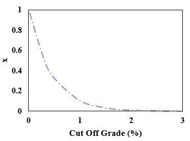
In Table 4, the model required variables are calculated using the values of Tables 1 and 2. Changes in these variables relative to the cutoff grade are shown in Figures 1 to 4. In Figure 1, the changes of the average grade compared to the cutoff grade are shown, which have a direct relationship with each other, and with the decrease of the cutoff grade, the average grade decreases. Figure 2 shows the changes in the ratio of the amount of ore to the total material inside the cavity in relation to the cutoff grade, which decreases with the increase of the cutoff grade. Figure 3 shows the changes in the ratio of the amount of product to the total material inside the cavity compared to the cutoff grade, which decreases with the increase of the cutoff grade. Figure 4 shows the changes in the ratio of the amount of product to the amount of ore in relation to the cutoff grade, which decreases with the decrease of the cutoff grade. To get the answer, first, the $g_{m h}, g_{h r}$ and $g_{m r}$ values must be calculated. According to the definition of $g_{m h}$ the corresponding cutoff grade is the point that there $x=H / M=0.5$. According to Table 4, this point is between the cutoff grades of 0.3 and 0.5%. By introspection, the approximate result below is obtained:
$g_{m h}=0.309 \%$
Table 2. Specifications for materials inside the cavity designed
|
Grade Average (%) |
Material Tonnage (thousand tons) |
Grade Range (%) |
|
3.55 2.78 2.27 1.75 1.24 0.73 0.40 0.14 |
35.31 72.97 226.07 692.27 2135.85 6567.10 5545.62 14724.81 |
> 3 2.5-3 2-2.5 1.5-2 1-1.5 0.5-1 0.3-0.5 < 0.3 |
Table 3. Economic and operational information of the mine
|
Amount |
Parameter |
|
90 % $1 per ton $2 per ton $0.5 per kilogram product $550 a year $1 per kilogram product 2.2 million tons per year 1.1 million tons per year 6600 tons per year |
Recovery ($y$) Mining cost ($m$) Processing cost ($h$) Refining cost ($r$) Fixed cost ($f$) Sales price ($S$) Mining Capacity ($M$) Processing Plant Capacity ($H$) Refining Capacity ($R$) |
Table 4. Information on model variables
|
$\frac{u}{x}$ |
$u\left(\frac{k g}{t}\right)$ |
$x$ |
$\bar{g}$ |
$Q_h$ |
$g_c$ |
|
31.95 27.31 22.68 18.04 13.41 8.78 6.92 4.14 |
0.037 0.098 0.253 0.617 1.414 2.845 3.524 4.140 |
0.001 0.004 0.011 0.034 0.105 0.325 0.509 1 |
3.55 3.035 2.52 2.005 1.49 0.975 0.769 0.46 |
35.31 108.28 334.35 1026.62 3162.47 9729.57 15275.19 30000 |
3 2.5 2 1.5 1 0.5 0.3 0 |
Similarly, by definition, $g_{hr}$ is the corresponding cutoff grade of the point that there $\frac{u}{x}=\frac{R}{H}=6$. According to Table 4, this point is between the cutoff grades of 0 and 0.3%. By interpolating, the approximate result below is obtained:
$g_{h r}=0.200 \%$
Similarly, by definition, $g_{hr}$ is the corresponding cutoff grade of the point that there $u=\frac{R}{M}=3$. According to Table 4, this point is between the cutoff grades of 0.3 and 0.5%. By interpolating, the approximate result below is obtained:
$g_{m r}=0.454 \%$
First, the problem is solved by the Lane method. According to the above relations [20, 22]:
$g_m=\frac{h}{y(p-r)}=0.244 ; g_h=\frac{h+\frac{F+f}{H}}{y(p-r)}=0.296 ; g_r=\frac{h}{y\left(p-r-\frac{F+f}{R}\right)}=0.26$
Figure 1. Average grade variations relative to the cutoff grade
Figure 2. Curve changes in the ratio of the amount of ore to total cavity material in relation to the cutoff grade
Figure 3. Curve changes in the ratio of the amount of product to total material within the cavity than the cutoff grade
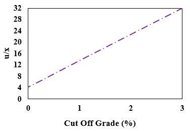
Figure 4. Changes in the ratio of the amount of product to the amount of ore relative to the cutoff grade
The result of the Lane method is shown in Table 5.
Table 5. Results of the calculation of the Lane algorithm
|
0.244% 0.296% 0.260% 0.309% 0.200% 0.454% |
$g_m$ $g_h$ $g_r$ $g_{mh}$ $g_{hr}$ $g_{mr}$ |
|
0.260% |
$g_{out}$ |
3.4 Problem solving by analytical method
To solve the problem in the method presented in this paper, by inserting balance grades values in the target function model 50, this model is as follows:
$\max P=\left\{\begin{array}{lr}P_m & g_c \geq 0.454 \\ P_h & g_c \leq 0.200 \\ P_r & 0.200 \leq g_c \leq 0.454\end{array}\right.$
Also, the three functions $P_m$ and $P_h$ and $P_r$, According the Eqs. (34), (37) and (40), the following relations are obtained:
$\begin{gathered}P_m=0.5 u-2 x-1.2 \\ P_h=0.5 u-2.5 x-1 \\ P_r=0.42 u-2 x-1\end{gathered}$
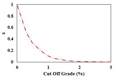
Table 6 shows the value of the target function in justified grade areas. The variation curve $P$ is relative to the cutoff grade in the maximum profit margin in Figure 5. The corresponding cutoff grade is the highest amount of profit, i.e., the optimal cutoff grade obtained by this method, is $g_out$=0.454%. Also, changes in the ratio of the amount of ore to total materials within the cavity and changes in the ratio of the amount of product to total material within the cavity are shown in Figures 6 and 7, respectively, which decrease with the increase in cutoff grade.
As can be seen, the optimum cutoff grade obtained in the Lane method is equivalent to the refining limiting cutoff grade ($g_r$=0.260), while the optimum cutoff grade obtained in this method is equal to the equilibrium cutoff grade of mining-refining ($g_mr$=0.454). The profit obtained from the optimal cutoff grade obtained in this method is about 20% more than the profit obtained from the optimal cutoff grade obtained by the Lane method [20, 22].
First, the problem is solved by the Lane method. According to the above relations:
$\begin{gathered}g_m=\frac{h}{y(p-r)}=0.244 \\ g_h=\frac{h+\frac{F+f}{H}}{y(p-r)}=0.296 \\ g_r=\frac{h}{y\left(p-r-\frac{F+f}{R}\right)}=0.26\end{gathered}$
0.5%. By interpolating, the approximate result below is obtained:
Table 6. The value of the objective function in the grade different ranges
|
$P$ Value |
$u$ |
$x$ |
Effective $P$ |
$g_c$ |
|
-1.164 -1.110 -0.970 -0.651 -0.003 1.004 1.374 1.243 1.145 0.950 0.640 |
0.075 0.196 0.505 1.234 2.827 5.708 6.016 7.050 7.214 7.460 8.280 |
0.001 0.004 0.011 0.034 0.105 0.325 0.367 0.509 0.574 0.672 1 |
$P_m$ $P_m$ $P_m$ $P_m$ $P_m$ $P_m$ $P_m$, $P_r$ $P_r$ $P_r$ $P_h$, $P_r$ $P_h$ |
3 2.5 2 1.5 1 0.5 0.454 0.3 0.260 0.200 0 |
Figure 5. Profit change curve relative to the cutoff grade
This problem is designed so that the values $\bar{g}$ and $x$ of Table 4 can be represented by the following mathematical equations (In these relationships, $g_c$ and $\bar{g}$ in percent, and $x$ in ton per ton):
$\begin{gathered}\bar{g}=1.03 g_c+0.46 \\ x=e^{-2.25 g_c}\end{gathered}$
as a result:
$u=y \cdot \bar{g} \cdot x=\left(9.27 g_c+4.14\right) e^{-2.25 g_c}$
These relationships are replaced in the three-dimensional objective functions:
$\begin{gathered}P_m=\left(9.27 g_c+2.14\right) e^{-2.25 g_c}-1.2 \\ P_h=\left(9.27 g_c+1.64\right) e^{-2.25 g_c}-1 \\ P_r=\left(7.79 g_c+1.48\right) e^{-2.25 g_c}-1\end{gathered}$
Figure 6. The changes curve of the ratio of the amount of ore to total material within the cavity relative to the cutoff grade
Figure 7. Changes curve in the ratio of the amount of product to total material within the cavity relative to the cutoff grade
The values of $g_m, g_h$, and $g_r$ are obtained with the zero equation, the derivation of the above functions is relative to the cutoff grade:
$\begin{aligned} & \frac{d P_m}{d g_c}=0 \Rightarrow g_m=0.425 \\ & \frac{d P_h}{d g_c}=0 \Rightarrow g_h=0.481 \\ & \frac{d P_r}{d g_c}=0 \Rightarrow g_r=0.466\end{aligned}$
As seen, the $g_m, g_h$, and $g_r$ values obtained here are different from values obtained from previous relationships. This difference arises from assume the constant $\bar{g}$ relative to ${g}_c$ in the Lane method. Final results obtained from the analytical solution method are shown in Table 7. In this table, the optimal cutoff grade is calculated from the 6th grade, selected by the Lane method.
Table 7. Results of the calculation of the analytical solution method
|
0.425% 0.481% 0.466% 0.309% 0.200% 0.454% |
$g_m$ $g_h$ $g_r$ $g_{mh}$ $g_{hr}$ $g_{mr}$ |
|
0.454% |
$g_{out}$ |
As can be seen, the optimum cutoff grade obtained by analytical method, like the method presented in this paper, is equivalent to the equilibrium mining-refining cutoff grade of 0.454%.
Optimization of the factory cutoff grade is one of the most important works is to be done at the stage of planning the production of open pit mines. This paper presents a new approach is presented to solving the Lane model, a classical method for determining the optimal factory cutoff grade. To do this, the problem was formulated according to the Lane model as a three-step process with mining capacity limitations, processing plant and refining. Then, by analyzing the relationships between the parameters and the model decision variables, an innovative method for its solution was developed. Finally, a numerical example was once solved by the method of Lane and once by the method presented in this paper and the results of these methods are compared and their validity was evaluated by solving the problem in an analytical method. In Lane model, the values of $g_m, g_h$, and $g_r$ are 0.244%, 0.296% and 0.26%, respectively, while in the new method they are 0.425%, 0.481% and 0.466% respectively, also, the equilibrium grades of $g_{m h}, g_{h r}$ and $g_{m r}$ were obtained as 0.309%, 0.2% and 0.454% respectively. In the Lane method, the optimal cutoff grade is 0.26%, while in the new method, the optimal cutoff grade is equal to 0.454%. Comparison of the economic results obtained from the two methods shows that the profit from the cutoff grade obtained in the new method is more than the profit from the calculated cutoff grade by the Lane method. This difference arises since in the Lane method, the value of $\bar{g}$ is assumed to be constant relative to ${g}_c$, while this was not so, and $\bar{g}$ is ascending strictly functional of ${g}_c$.
[1] Minnitt, R. (2004). Cut-off grade determination for the maximum value of a small Wits-type gold mining operation. Journal of the Southern African Institute of Mining and Metallurgy, 104: 277-283.
[2] Abdollahisharif, J., Bakhtavar, E., Anemangely, M. (2012). Optimal cut-off grade determination based on variable capacities in open-pit mining. Journal of the Southern African Institute of Mining and Metallurgy, 112: 1065-1069.
[3] Shinkuma, T., Nishiyama, T. (2000). The grade selection rule of the metal mines; An empirical study on copper mines. Resources Policy, 26(1): 31-38. https://doi.org/10.1016/S0301-4207(00)00014-3
[4] Ahmadi, M.R. (2018). Cutoff grade optimization based on maximizing net present value using a computer model. Journal of Sustainable Mining, 17(2): 68-75. https://doi.org/10.1016/j.jsm.2018.04.002
[5] Asad, M. (2007). Optimum cut-off grade policy for open pit mining operations through net present value algorithm considering metal price and cost escalation. Engineering Computations, 24(7): 723-736. https://doi.org/10.1108/02644400710817961
[6] Asad, M., Dessureault, S. (2005). Cutoff grade optimization algorithm for open pit mining operations with consideration of dynamic metal price and cost escalation during mine life. In Proceedings of the 32nd International Symposium on Application of Computers & Operations Research in the Mineral Industry, pp. 273-277.
[7] Rahimi, E., Ghasemzadeh, H. (2015). A new algorithm to determine optimum cut-off grades considering technical, economical, environmental and social aspects. Resources Policy, 46: 51-63. https://doi.org/10.1016/j.resourpol.2015.06.004
[8] Asad, M., Topal, E. (2011). Net present value maximization model for optimum cut-off grade policy of open pit mining operations. Journal of the Southern African Institute of Mining and Metallurgy, 111(11): 741-750.
[9] Azimi, Y., Osanloo, M., Esfahanipour, A. (2012). Selection of the open pit mining cut-off grade strategy under price uncertainty using a risk based multi-criteria ranking system. Archives of Mining Sciences, 57(3): 741-768. https://doi.org/10.2478/v10267-012-0048-8
[10] Bascetin, A., Nieto, A. (2007). Determination of optimal cut-off grade policy to optimize NPV using a new approach with optimization factor. Journal-South African Institute of Mining and Metallurgy, 107(2): 87.
[11] Osanloo, M., Ataei, M. (2003). Using equivalent grade factors to find the optimum cut-off grades of multiple metal deposits. Minerals Engineering, 16(8): 771-776. https://doi.org/10.1016/S0892-6875(03)00163-8
[12] Cairns, R.D., Shinkuma, T. (2003). The choice of the cutoff grade in mining. Resources Policy, 29(3-4): 75-81. https://doi.org/10.1016/j.resourpol.2004.06.002
[13] Cetin, E., Dowd, P. (2016). Multiple cut-off grade optimization by genetic algorithms and comparison with grid search method and dynamic programming. Journal of the Southern African Institute of Mining and Metallurgy, 116(7): 681-688. http://doi.org/10.17159/2411-9717/2016/v116n7a10
[14] Gholamnejad, J. (2008). Determination of the optimum cutoff grade considering environmental cost. J. Int. Environmental Application & Science, 3(3): 186-194.
[15] Gholinejad, M., Moosavi, E. (2016). Optimal mill cut-off grade modeling in the mineral deposits via MIP: Haftcheshmeh copper deposit. Journal of Mining Science, 52: 732-739. https://doi.org/10.1134/S1062739116041142
[16] Hustrulid, W.A., Kuchta, M., Martin, R.K. (2013). Open Pit Mine Planning and Design, Two Volume Set & CD-ROM Pack. CRC Press.
[17] Jafarnejad, A. (2012). The effect of price changes on optimum cut-off grade of different open-pit mines. Journal of Mining and Environment, 3(1): 61-68. https://doi.org/10.22044/jme.2012.75
[18] Ahmadi, M.R., Shahabi, R.S. (2018). Cutoff grade optimization in open pit mines using genetic algorithm. Resources Policy, 55: 184-191. https://doi.org/10.1016/j.resourpol.2017.11.016
[19] Jafarnejad, A., Khodaiari, A.A. (2008). A new method for solving the Lane model to determine the optimal factory cutoff grade. Iranian Journal of Mining Engineering (IRJME), 3: 1-10.
[20] Lane, K.F. (1964). Choosing the optimum cut-off grade Q. Colorado Sch. Min., 59: 811-829.
[21] Azimi, Y., Osanloo, M. (2011). Determination of open pit mining cut-off grade strategy using combination of nonlinear programming and genetic algorithm. Archives of Mining Sciences, 56(2): 189-212.
[22] Lane, K.F. (1988). The Economic Definition of Ore: Cut-Off Grades in Theory and Practice. Mining Journal Books.
[23] Mohammadi, S., Kakaie, R., Ataei, M., Pourzamani, E. (2017). Determination of the optimum cut-off grades and production scheduling in multi-product open pit mines using imperialist competitive algorithm (ICA). Resources Policy, 51: 39-48. https://doi.org/10.1016/j.resourpol.2016.11.005
[24] Osanloo, M., Rashidinejad, F., Rezai, B. (2008). Incorporating environmental issues into optimum cut-off grades modeling at porphyry copper deposits. Resources Policy, 33(4): 222-229. https://doi.org/10.1016/j.resourpol.2008.06.001
[25] Rashidinejad, F., Osanloo, M., Rezai, B. (2008). An environmental oriented model for optimum cut-off grades in open pit mining projects to minimize acid mine drainage. International Journal of Environmental Science & Technology, 5: 183-194. https://doi.org/10.1007/BF03326012
[26] Shinkuma, T. (2000). A generalization of the Cairns–Krautkraemer model and the optimality of the mining rule. Resource and Energy Economics, 22(2): 147-160. https://doi.org/10.1016/S0928-7655(99)00020-2
[27] Taylor, H. (1972). General background theory of cut-off grades. Transactions of the Institute of Mining and Metallurgy 96, A204-A216.
[28] Taylor, H. (1985). Cutoff grades-some further reflections. Institution of Mining and Metallurgy Transactions. Section A. Mining Industry 94.