Nidal Adnan Jasim*![]() | Abdulrahman Adnan Ibrahim
| Abdulrahman Adnan Ibrahim![]() | Wadhah Amer Hatem
| Wadhah Amer Hatem![]()
©2023 IIETA. This article is published by IIETA and is licensed under the CC BY 4.0 license (http://creativecommons.org/licenses/by/4.0/).
OPEN ACCESS
Although earned value management (EVM) offers considerable advantages for schedule and cost control within oil projects, its implementation as a project control technique remains limited in Iraq. This study primarily aims to establish predictive models, utilizing support vector machine (SVM), to estimate earned value performance indicators namely schedule performance index (SPI), cost performance index (CPI), and to-complete cost performance index (TCPI) within the context of Iraqi oil projects. The dataset, encompassing 83 monthly reports spanning from 26th June 2015 to 25th August 2022, was sourced from the Karbala Refinery Project. This project, managed by the oil projects company (SCOP) under the Iraqi Ministry of Oil, represents one of the largest and most contemporary initiatives within the region. The results revealed significant findings, including an average accuracy (AA%) for CPI, SPI, and TCPI of 96.093%, 91.709%, and 66.024%, respectively. Correlation coefficients (R) were registered at 92.8%, 98.2%, and 93.3%, while the root mean squared error (RMSE) stood at 0.0969, 0.0604, and 0.2260 respectively. In conclusion, the SVM technique was employed in this study to derive predictive models, yielding superior accuracy for earned value indexes.
earned value management, oil projects, Iraq, support vector machine, performance indicators, predictive models
Oil and gas construction projects play a pivotal role in facilitating production processes within the industry [1]. However, these projects frequently grapple with protracted risks, resulting in extended timelines, elevated costs, and compromised quality, thereby undermining their success [1]. The inherent complexity of technology and management within the oil and gas sector renders these projects among the most challenging to execute. For project managers, in addition to possessing relevant experience, adherence to a consistent reference framework predicated on the continual monitoring and evaluation of all formal project stages is essential [2]. Effective management within the oil and gas industry necessitates robust strategies for time, cost, and quality, thereby underscoring the need for techniques to mitigate the risk of future project failures [2].
EVM, a prevalent approach for project monitoring and control, facilitates project progress analysis by measuring scope, schedule, and cost [3]. Despite its benefits, the current methodologies and strategies for estimating earned value indexes in Iraq are deemed subpar and inefficient. The demand for novel and advanced technologies that enable the timely, accurate, and flexible estimation of earned value indexes has thus intensified [4]. Given the absence of an established modern methodology for estimating the earned value of Iraq's oil projects, this study primarily aims to formulate three mathematical models, leveraging the Support Vector Machine, to predict the key indicators of earned value in the construction of the Karbala Refinery Project. These performance indicators are CPI, SPI, and TCPI.
Numerous researchers have explored employing SVM techniques for project management, focusing specifically on maintaining cost and timeline control. For instance, a SVM model was developed by Hasan et al. to estimate the cost of road projects, utilizing 43 sets of bills of quantity collated from Baghdad, Iraq [5]. The prediction equations formulated within this model demonstrated a robust performance in estimating construction costs for roads in Baghdad city, posting an average accuracy (AA) of 99.65% and a coefficient of determination (R²) of 97.63% [5].
Similarly, Juszczyk developed a model founded on machine learning and SVM techniques to predict site overhead costs, with the results affirming its effectiveness [6]. Alawadi et al. proposed an SVM-based model to furnish preliminary budget estimates for bridge construction, using basic data and metrics about bridges in the initial construction stages as input [7]. The forecasts derived from this model exhibited an acceptable estimation error range of 25-30%, indicating reasonable accuracy [7].
Additionally, a mathematical model was developed to predict the optimal time of completion for repetitive construction projects [8]. The constructed model, which leveraged SVM techniques, demonstrated a significant capability to predict the time of repetitive construction projects (RCPs), with a correlation coefficient of 97%, a mean absolute error (MAE) of 3.6, and a RMSE of 7% [8].
Eltoukhy and Nassar employed SVM to develop a model for predicting cost and time overruns in construction projects, by elucidating the causes and effects of cost and schedule overruns in building projects [9]. In 2021, Chandanshive and Kambekar developed a cost prediction model to enable accurate cost predictions early in a project's lifecycle [10]. The resultant SVM model for cost prediction in building construction projects exhibited a correlation coefficient (R) of 97.5257% and an R² of 94.299% between the actual and expected cost, with the overall accuracy defined as 94.29%. The mean absolute percent error (MAPE) of 8.96% signified that the model's percentage error met the error requirements [10].
Notably, Susilowati and Kurniaji integrated EVM methodology into a development project encompassing malls and hotels, measuring performance through indicators such as the cost performance index (CPI), and the schedule performance index (SPI) [11]. Hussien and Jasim proposed a tool that melds the building information modelling (BIM) technique with EVM, offering several features that assist project managers in circumventing errors during project progress stages by identifying conflicting elements that induce time delays and cost deviations [12].
To determine the factors that affect and develop mathematical equations to quickly and readily determine the indexes, the following steps can be used to achieve this goal:
Figure 1 shows the methodology for development of SVM models.
Figure 1. Methodology of research
The project of Karbala Refinery is selected as a case study to achieve the goal of the research being one of the huge projects, project Location is 25 km South of Karbala City, Iraq (100 km South of Baghdad City). The total site area is (10 km2) including the Refinery area is (6 km2). The total cost of this project is about (USD 6,641,089,012), with a working duration of (54 months). More information is summarized in Table 1. Figure 2 displays the units’ diagram for the Karbala Refinery project as well as Figure 3 shows a 3D picture and the site photo of the Crude & Vacuum Distillation Unit.
Table 1. Project background information
|
Item Name |
Details |
|
Project Name |
Karbala Refinery Project |
|
Project Location |
25km South of Karbala City, Iraq (100km South of Baghdad City) |
|
Employer |
State Company for Oil Projects (SCOP)/Oil Ministry |
|
Contractor |
The Korean Consortium Headed by Hyundai HDGSK JV(HDEC+GS+SK+HEC) |
|
Consultant |
TechnipFMC |
|
Refinery Area |
3km×2km |
|
Site Area |
5km×2km |
|
Production Capacity |
140,000 BPSD |
|
Type of Contract |
EPC (design, purchase, and construction) |
|
Contract Signing Date (EPC) |
15/4/2014 |
|
Actual start date |
28/5/2014 |
|
Duration of the Original Contract |
54 Months |
|
Planned Completion Date |
16/2/2022+1 year (trial operation) |
|
Expected Completion Date |
31/7/2023 |
|
Contract Amount |
6,641,089,012 $ |
|
The Value of the Original Contract |
6,023,000,000 $ |
|
FEED Contractor |
Technip Italy S.p.A(2009-2010) |
|
Licensors |
UOP, Axens, Haldor Topsoe, Poener, Tecnimont |
Figure 2. Units diagram of Karbala Refinery Project
Figure 3. Crude and vacuum distillation unit
All reports of the Karbala refinery project have been obtained from the Karbala Refinery Project Authority, the state company for oil projects (SCOP), Iraqi Ministry of Oil, which (83) reports. (73) reports from it used for building the (SVM) models and, (10) used for generalization. For each one of the three models (CPI, SPI, TCPI), the data is separated into three categories (training, testing, and validation). The CPI model got 78% of the data in the training set, 11% in the test set, and 11% in the validation set. As a result, (57) reports were used for training, (8) for validation, and (8) for testing this model. While the SPI model received 70% of the data from the training set, the test set received 5% and the validation set received 25%. As a consequence, (51) reports were used for training, (18) for validation, and (4) for testing. As for the TCPI model the optimal division was found to be 84% for the training dataset, 5% for the testing dataset, and 11% for the validation datasets, as a consequence (61) reports were used for training, (8) for verification, and (4) for testing. The precision of all these divisions was based on the lowest testing errors and highest Correlation Coefficients (r) value.
Today, support vector machine applications are used for solving many engineering problems such as earned value predicting. The researcher studied many support vector machine programs such as Win SVM, MATLAB SVM Toolbox, LIBSVM, SVM light, STATISTICA, DTREG and WEKA. The present study made use of the WEKA Software because of the researcher found that the best software for support vector machine, which is easy to apply and has a high compatibility with both simple and more complex issues, and can accept different kinds of variables and factors. Weka is a set of state-of-the-arts ML algorithms and data pre-processing tool, which was developed by Waikato University, New Zealand. WEKA is short for Waikato environment for knowledge analysis, and its design enables a flexible and easy check of currently applied methods on data sets. Third edition of Weka was used in this study since the best stable version of Weka. There are five steps involved for the implementation of SVM using Weka, namely Data Division, SMOreg, function selecting, kernel selection, and determining the learning SVM parameters. As for the work presented in this chapter, the lowest root mean square error (RMSE) was adopted based on the Kernel and SVM parameters (C and epsilon).
The SVM model requires lots of information and data, which was collected from the Karbala Refinery Project for the period from 2015 to 2022. The data collection method used in this paper is direct data collection, as the project data was obtained from the Karbala Refinery Project Authority after many approvals, interviews and repeated visits to the project. Despite the fact that this method is somewhat complicated, a sufficient amount of reliable data has been collected from documents and reports on the planning and implementation of the refinery. Historical data contained both dependent and independent variables that were chosen and identified from (83) reports for the Karbala Refinery project. Three variables have been identified as being dependent, namely the Cost Performances Indicator (CPI), Schedule Performances Indicator (SPI), and To-Complete Cost Performances Indicator (TCPI) and six variables were chosen as being independent as following:
The variables used in the SVM models that affect the EV index are shown in Table 2.
Table 2. Variables of SVM models
|
Parameters |
Input Values |
|||||
|
BAC(USD) |
AC(USD) |
A% |
EV(USD) |
P% |
PV(USD) |
|
|
N |
83 |
83 |
83 |
83 |
83 |
83 |
|
Range |
0 |
1,725,290,950 |
0.987 |
1,773,593,250 |
0.985 |
1,770,717,250 |
|
Minimum |
1,797,500,000 |
5,392,500 |
0.005 |
8,088,750 |
0.015 |
26,782,750 |
|
Maximum |
1,797,500,000 |
1,730,683,450 |
0.991 |
1,781,682,000 |
1.000 |
1,797,500,000 |
|
Mean |
1,797,500,000 |
798,844,121 |
0.496 |
890,884,313 |
0.782 |
1,406,171,256 |
|
St. D |
0 |
611,143,561 |
0.358 |
642,934,013 |
0.324 |
581,851,806 |
|
|
Output Values |
|||||
|
CPI |
SPI |
TCPI |
||||
|
N |
83 |
83 |
83 |
|||
|
Range |
0.597 |
0.872 |
0.820 |
|||
|
Minimum |
1.029 |
0.201 |
0.178 |
|||
|
Maximum |
1.626 |
1.073 |
0.998 |
|||
|
Mean |
1.177 |
0.606 |
0.771 |
|||
|
St. D |
0.148 |
0.320 |
0.240 |
|||
To guarantee ensures all variables receive the same attention throughout training, the input and output variables are pre-processed by scaling them to eliminate their dimension. As part of this approach, scaled values with a minimum and maximum of (x min/x max) are computed for each variable in Eq. (1):
Scale Value $=\frac{X-X_{\min }}{X_{\max }-X_{\min }}$ (1)
It is necessary for SVM models to be organized, so as to improve the performance. The main factors to be addressed are developing model input, data divisions, and preprocessing, developing the model architecture, and its optimization (training), stop criteria, and model validation. A structured methodology is applied to develop the model, which involves four major phases:
The same variables defined at the data identifying step are used for developing the three mathematical SVM models, using the project characteristics to predict the EV indexes. Through the third version of Weka, the following models were developed:
8.1 Cost performance index (CPI) model
This model's development involves the following five steps:
8.1.1 Data division CPI model
The data is divided into three sets, namely training, testing, and validating sets as shown in Table 3.
Table 3. Impact of data split on performance of CPI model
|
Data Set |
Statistical Parameters |
Input Variables |
Output |
|||||
|
P% |
BCWS |
A% |
BCWP |
ACWP |
BAC |
CPI |
||
|
Training
n=57 |
Range |
0.9851 |
1770717250 |
0.9867 |
1773593250 |
1717202200 |
0 |
0.5650 |
|
Minimum |
0.0149 |
26782750 |
0.0045 |
8088750 |
5392500 |
1797500000 |
1.0340 |
|
|
Maximum |
1.0000 |
1797500000 |
0.9912 |
1781682000 |
1722594700 |
1797500000 |
1.5990 |
|
|
Mean |
0.7741 |
1391507820 |
0.4724 |
849066469 |
758133077 |
1797500000 |
1.1855 |
|
|
St. Deviation |
0.3370 |
605735060 |
0.3547 |
637521603 |
602944073 |
0 |
0.1513 |
|
|
Testing
n=8 |
Range |
0.9509 |
1709242750 |
0.9568 |
1719848000 |
1655250180 |
0 |
0.3500 |
|
Minimum |
0.0491 |
88257250 |
0.0207 |
37208250 |
26671250 |
1797500000 |
1.0450 |
|
|
Maximum |
1.0000 |
1797500000 |
0.9775 |
1757056250 |
1681921430 |
1797500000 |
1.3950 |
|
|
Mean |
0.7633 |
1371964344 |
0.4714 |
847341500 |
751552641 |
1797500000 |
1.1818 |
|
|
St. Deviation |
0.3620 |
650610737 |
0.3817 |
686023075 |
645018042 |
0 |
0.1277 |
|
|
Validation
n=8 |
Range |
0.8742 |
1571374500 |
0.9102 |
1636084500 |
1641147940 |
0 |
0.5970 |
|
Minimum |
0.1258 |
226125500 |
0.0810 |
145597500 |
89535510 |
1797500000 |
1.0290 |
|
|
Maximum |
1.0000 |
1797500000 |
0.9912 |
1781682000 |
1730683450 |
1797500000 |
1.6260 |
|
|
Mean |
0.8568 |
1540098000 |
0.6391 |
1148714844 |
1058329529 |
1797500000 |
1.1690 |
|
|
St. Deviation |
0.3103 |
557694339 |
0.3863 |
694445675 |
682027724 |
0 |
0.1979 |
|
8.1.2 Selection kernel CPI model
The next step is to choose the kernel, as displayed in Table 4. The poly-kernel was chosen as the optimal kernel for the CPI model because its root mean square error (RMSE) is equal to 0.1, which is the least number found.
Table 4. Effects of the kernel function on CPI model
|
Kernel Type |
MAE |
RMSE |
Correlation Coefficient % |
|
Normalised poly-kernel |
0.0917 |
0.1434 |
72.79 |
|
Poly-kernel |
0.0717 |
0.1 |
74.34 |
|
RBF kernel |
0.0855 |
0.1301 |
63.89 |
8.1.3 Selection of the SVM parameters (C and epsilon) for the CPI model
Table 5 illustrates an example of the C effect on the CPI model. When the C value is 10 the greatest (r) value is (96.98%), the mean absolute error (MAE) is (0.0354), and the least RMSE is (0.0786) making this the ideal value. According to the statistics in this table, changes in C, especially those falling between (1 to 10), have little impact on the performance of the CPI models. This supports including it in the study's suggested model.
Table 5. Impact of changing parameter C on CPI model performance
|
Parameter (C) |
MAE |
RMSE |
Coefficient Correlation (%) |
|
1 |
0.0717 |
0.1 |
74.34 |
|
2 |
0.0641 |
0.0905 |
80.4 |
|
3 |
0.0616 |
0.0861 |
82.56 |
|
4 |
0.0601 |
0.0833 |
83.86 |
|
5 |
0.0568 |
0.0779 |
86.04 |
|
6 |
0.0535 |
0.0748 |
86.97 |
|
7 |
0.0529 |
0.0746 |
86.98 |
|
8 |
0.0529 |
0.0745 |
86.98 |
|
9 |
0.0529 |
0.0745 |
86.99 |
|
10 |
0.0528 |
0.0745 |
86.99 |
Table 6 displays Epsilon's impact on the CPI model. Considering that the greatest (r) value is (87.06%), the smallest RMSE is (0.0744), and the mean absolute error (MAE) is (0.0528) Epsilon is considered to be at its best when it is valued equal to (0.006). The information in this table demonstrates that variations in Epsilon have little impact on the functionality of CPI models, especially when they fall between (0.001 to 0.05). This is in favor of including it in the study's model.
Table 6. Impact of changing parameter Epsilon on CPI model performance
|
Parameter Epsilon |
MAE |
RMSE |
Coefficient Correlation (%) |
|
0.001 |
0.0528 |
0.0745 |
86.99 |
|
0.002 |
0.0528 |
0.0745 |
86.99 |
|
0.003 |
0.0528 |
0.0746 |
87.01 |
|
0.004 |
0.0527 |
0.0745 |
87.02 |
|
0.005 |
0.0528 |
0.0745 |
87.04 |
|
0.006 |
0.0528 |
0.0744 |
87.06 |
|
0.007 |
0.0528 |
0.0745 |
87.06 |
|
0.008 |
0.0528 |
0.0745 |
87.06 |
|
0.009 |
0.0528 |
0.0747 |
87.06 |
|
0.01 |
0.0528 |
0.0747 |
87.06 |
|
0.02 |
0.0531 |
0.0749 |
87.08 |
|
0.03 |
0.0534 |
0.0752 |
87 |
|
0.04 |
0.054 |
0.0759 |
86.97 |
|
0.05 |
0.0552 |
0.0768 |
86.83 |
8.1.4 Equation of CPI model
Table 7 shows the connection weights collected by the Weka software for the optimal CPI model. A scale is not necessary because the program decides whether or if the data should be transformed as well as the method of transformation.
Table 7. Weight estimates for model CPI
|
Layer |
Wji, (Weight from Node I in the Input Layer to Node J in the Hidden Layer) |
||||
|
Input |
P% |
BCWS |
A% |
BCWP |
ACWP |
|
Weights |
-0.2287 |
-0.2287 |
1.5477 |
1.5477 |
-3.2236 |
|
Bias |
0.55889 |
||||
By using the connection weights and threshold level stated in Table 6, the CPI value might be predicted in the following method:
$\mathrm{CPI}_{\text {nor }}=0.5589 -(0.2287 \times \mathrm{P} \%) -(0.2287 \times \mathrm{BCWS}) +(1.5477 \times \mathrm{A} \%) +(1.5477 \times \mathrm{BCWP}) -(3.2236 \times \mathrm{ACWP})$ (2)
$\mathrm{CPI}_{\text {act }}=\mathrm{CPI}_{\text {nor }} \times \mathrm{range}+\mathrm{min}$ (3)
$\mathrm{CPI}_{\text {act }}=\mathrm{CPI}_{\text {nor }} \times 0.5650+1.0340$ (4)
The above-mentioned equation's implementation can be clarified by utilizing the data used in the SVM model training for CPI, as shown in report no.66 in Table 8. The predicted value obtained from the above equation equals (1.071), which, when compared to the real value measured by hand (CPI=1.064), is relatively accurate. These value variations are considered as minor. Before utilizing Eq. (2) it should be noted that all input variables must be transformed to values between (0-1) because Eq. (2) was built using Eq. (1). To obtain actual data out from normalized ones, conversions to actual values were made using Eq. (4) and Table 3.
Table 8. Verification of CPI model
|
Report No. |
(P%) |
PV(BCWS) |
(A%) |
EV(BCWP) |
AC(ACWP) |
Actual CPI |
Predicted CPI |
Residual |
|
66 |
1.000 |
1,797,500,000 |
0.920 |
1,653,879,750 |
1,554,648,510 |
1.064 |
1.071 |
-0.007 |
|
67 |
1.000 |
1,797,500,000 |
0.966 |
1,736,924,250 |
1,661,250,180 |
1.046 |
1.040 |
0.006 |
|
68 |
0.126 |
226,125,500 |
0.081 |
145,597,500 |
89,535,510 |
1.626 |
1.367 |
0.259 |
|
69 |
0.729 |
1,309,658,500 |
0.177 |
318,517,000 |
285,321,330 |
1.116 |
1.172 |
-0.055 |
|
70 |
1.000 |
1,797,500,000 |
0.303 |
543,743,750 |
448,796,070 |
1.212 |
1.149 |
0.062 |
|
71 |
1.000 |
1,797,500,000 |
0.742 |
1,332,846,250 |
1,104,744,180 |
1.206 |
1.232 |
-0.025 |
|
72 |
1.000 |
1,797,500,000 |
0.933 |
1,676,528,250 |
1,591,657,000 |
1.053 |
1.054 |
-0.001 |
|
73 |
1.000 |
1,797,500,000 |
0.991 |
1,781,682,000 |
1,730,683,450 |
1.029 |
1.010 |
0.019 |
8.1.5 Verification of the CPI model
Table 8 summarizes and compares the CPI computation using SVM to validate the estimation model. It comprises the real CPI value received from the Karbala Refinery Project, as well as the estimated CPI value calculated using the SVM equation (as obtained from Weka V.3).
Figure 4. Comparison of predicted and actual for CPI model
Figure 4 illustrates the predicted values against the actual values for the verification data to show the capacity of the SVM model for CPI to assess the model. It is clear from this figure that the (R2=86.1%). The ten spare data that have not yet been used in any subset can have their earned value index predicted using the trained SVM models. The generalization results of the CPI model with (R2=82.03%) are excellent, as illustrated in Figure 5.
Figure 5. Generalization of CPI model
8.2 Schedule performance index (SPI) model
This model's development involves the following five steps:
8.2.1 Data division SPI model
The data is divided into three sets, namely training, testing, and validating sets, as show in Table 9.
Table 9. Impact of data split on performance of SPI model
|
Data set |
Statistical Parameters |
Input Variables |
Output |
|||||
|
P% |
BCWS |
A% |
BCWP |
ACWP |
BAC |
SPI |
||
|
Training
n=51 |
Range |
0.9851 |
1770717250 |
0.9867 |
1773593250 |
1717202200 |
0 |
0.8380 |
|
Minimum |
0.0149 |
26782750 |
0.0045 |
8088750 |
5392500 |
1797500000 |
0.2030 |
|
|
Maximum |
1.0000 |
1797500000 |
0.9912 |
1781682000 |
1722594700 |
1797500000 |
1.0410 |
|
|
Mean |
0.7517 |
1351159603 |
0.4634 |
832972074 |
747391901 |
1797500000 |
0.5833 |
|
|
St. Deviation |
0.3487 |
626752140 |
0.3630 |
652569381 |
618538507 |
0 |
0.3158 |
|
|
Testing
n=4 |
Range |
0.0012 |
2157000 |
0.4418 |
794135500 |
529322205 |
0 |
0.4420 |
|
Minimum |
0.9988 |
1795343000 |
0.2109 |
379092750 |
350235075 |
1797500000 |
0.2110 |
|
|
Maximum |
1.0000 |
1797500000 |
0.6527 |
1173228250 |
879557280 |
1797500000 |
0.6530 |
|
|
Mean |
0.9997 |
1796960750 |
0.3940 |
708125125 |
562434105 |
1797500000 |
0.3940 |
|
|
St. Deviation |
0.0006 |
1078500 |
0.2047 |
368017702 |
241926155 |
0 |
0.2049 |
|
|
Validation
n=18 |
Range |
0.9509 |
1709242750 |
0.9705 |
1744473750 |
1704012200 |
0 |
0.8470 |
|
Minimum |
0.0491 |
88257250 |
0.0207 |
37208250 |
26671250 |
1797500000 |
0.2020 |
|
|
Maximum |
1.0000 |
1797500000 |
0.9912 |
1781682000 |
1730683450 |
1797500000 |
1.0490 |
|
|
Mean |
0.8195 |
1473081208 |
0.5888 |
1058397958 |
962551076 |
1797500000 |
0.6867 |
|
|
St. Deviation |
0.3126 |
561817435 |
0.3712 |
667247781 |
643143526 |
0 |
0.3199 |
|
8.2.2 Selection kernel SPI model
The next step is to choose the kernel, as displayed in Table 10. The poly-kernel was chosen as the optimal kernel for the SPI model because its root mean square error (RMSE) is equal to (0. 0788), which is the least number found.
Table 10. Effects of the kernel function on SPI model
|
Kernel Type |
MAE |
RMSE |
Correlation Coefficient % |
|
Normalised poly-kernel |
0.0343 |
0.0883 |
97.62 |
|
Poly-kernel |
0.0356 |
0.0788 |
96.97 |
|
RBF kernel |
0.1361 |
0.1595 |
92.04 |
8.2.3 Selection of the SVM parameters (C and epsilon) for the SPI model
Table 11 illustrates an example of the C effect on the SPI model. When the C value is 6 the greatest (r) value is (96.98%), the MAE is (0.0354), and the least RMSE is (0.0786) making this the ideal value. According to the statistics in this table, changes in C, especially those falling between (1 to 10), have little impact on the performance of the SPI models. This supports including it in the study's suggested model.
Table 11. Effect of the parameter C in SVM model performance
|
Parameter (C) |
MAE |
RMSE |
Coefficient Correlation (%) |
|
1 |
0.0356 |
0.0788 |
96.97 |
|
2 |
0.0355 |
0.0786 |
96.97 |
|
3 |
0.0354 |
0.0787 |
96.97 |
|
4 |
0.0355 |
0.0786 |
96.97 |
|
5 |
0.0354 |
0.0787 |
96.97 |
|
6 |
0.0354 |
0.0786 |
96.98 |
|
7 |
0.0354 |
0.0787 |
96.97 |
|
8 |
0.0354 |
0.0786 |
96.97 |
|
9 |
0.0354 |
0.0786 |
96.98 |
|
10 |
0.0354 |
0.0787 |
96.97 |
Table 12 displays Epsilon's impact on the SPI model. Considering that the greatest (r) value is (97.35%), the smallest RMSE is (0.0717), and MAE is (0.0478), Epsilon is considered to be at its best when it is valued equal to (0.006). The information in this table demonstrates that variations in Epsilon have little impact on the functionality of SPI models, especially when they fall between (0.001 to 0.05). This is in favor of including it in the study's model.
Table 12. Impact of changing parameter Epsilon on SPI model performance
|
Parameter Epsilon |
MAE |
RMSE |
Coefficient Correlation (%) |
|
0.001 |
0.0354 |
0.0786 |
96.98 |
|
0.002 |
0.0356 |
0.0783 |
96.99 |
|
0.003 |
0.0358 |
0.0781 |
96.99 |
|
0.004 |
0.0361 |
0.0776 |
97.02 |
|
0.005 |
0.0363 |
0.0773 |
97.03 |
|
0.006 |
0.0365 |
0.0772 |
97.03 |
|
0.007 |
0.0368 |
0.0768 |
97.05 |
|
0.008 |
0.0369 |
0.0766 |
97.06 |
|
0.009 |
0.0372 |
0.0767 |
97.06 |
|
0.01 |
0.0374 |
0.0766 |
97.05 |
|
0.02 |
0.0396 |
0.0742 |
97.17 |
|
0.03 |
0.0423 |
0.0725 |
97.26 |
|
0.04 |
0.0448 |
0.0719 |
97.3 |
|
0.05 |
0.0478 |
0.0717 |
97.35 |
8.2.4 Equation of SPI model
The SPI value might be estimated using the connection weights and threshold level shown in Table 13 as follows:
Table 13. Weight estimates for model SPI
|
Layer |
Wji, (Weight from Node I in the Input Layer to Node J in the Hidden Layer) |
||||
|
Input |
P% |
BCWS |
A% |
BCWP |
ACWP |
|
Weights |
-0.3011 |
-0.3011 |
0.7557 |
0.7557 |
-0.2038 |
|
Bias |
0.2858 |
||||
By using the connection weights and threshold level shown in Table 12, the SPI value could be predicted in the following method:
$\mathrm{SPI}_{\mathrm{nor}}=0.2858-(0.3011 \times \mathrm{P} \%)-(0.3011 \times \mathrm{BCWS}) +(0.7557 \times \mathrm{A} \%) +(0.7557 \times \mathrm{BCWP})(0.2038 \mathrm{ACWP})$ (5)
$\mathrm{SPI}_{\mathrm{act}}=\mathrm{SPI}_{\text {nor }} \times \mathrm{range} +\mathrm{min}$ (6)
$\mathrm{SPI}_{\mathrm{act}}=\mathrm{SPI}_{\text {nor }} \times 0.8380+0.2030$ (7)
Table 14. Verification of SPI model
|
Report No. |
P% |
PV(BCWS) |
A%) |
EV(BCWP) |
AC(ACWP) |
Actual SP |
Predicted SPI |
Residual |
|
56 |
0.791 |
1,421,463,000 |
0.817 |
1469096750 |
1,356,613,950 |
1.034 |
0.954 |
0.080 |
|
57 |
1.000 |
1,797,500,000 |
0.898 |
1613615750 |
1,490,248,070 |
0.898 |
0.937 |
-0.039 |
|
58 |
1.000 |
1,797,500,000 |
0.951 |
1709782000 |
1,625,839,430 |
0.951 |
0.992 |
-0.041 |
|
59 |
1.000 |
1,797,500,000 |
0.978 |
1757056250 |
1,681,921,430 |
0.978 |
1.020 |
-0.042 |
|
60 |
0.049 |
88,257,250 |
0.021 |
37208250 |
26,671,250 |
0.422 |
0.444 |
-0.022 |
|
61 |
0.381 |
683,948,750 |
0.133 |
239427000 |
203,896,530 |
0.35 |
0.401 |
-0.051 |
|
62 |
0.950 |
1,708,164,250 |
0.192 |
344580750 |
312,585,420 |
0.202 |
0.173 |
0.029 |
|
63 |
1.000 |
1,797,500,000 |
0.242 |
434815250 |
387,053,895 |
0.242 |
0.205 |
0.037 |
|
64 |
1.000 |
1,797,500,000 |
0.493 |
886347250 |
669,708,990 |
0.493 |
0.499 |
-0.006 |
|
65 |
0.726 |
1,305,344,500 |
0.762 |
1369515250 |
1,104,744,180 |
1.049 |
0.941 |
0.108 |
|
66 |
1.000 |
1,797,500,000 |
0.920 |
1653879750 |
1,554,648,510 |
0.92 |
0.959 |
-0.039 |
|
67 |
1.000 |
1,797,500,000 |
0.966 |
1736924250 |
1,661,250,180 |
0.966 |
1.008 |
-0.042 |
|
68 |
0.126 |
226,125,500 |
0.081 |
145597500 |
89,535,510 |
0.644 |
0.476 |
0.168 |
|
69 |
0.729 |
1,309,658,500 |
0.177 |
318517000 |
285,321,330 |
0.243 |
0.271 |
-0.028 |
|
70 |
1.000 |
1,797,500,000 |
0.303 |
543743750 |
448,796,070 |
0.303 |
0.276 |
0.027 |
|
71 |
1.000 |
1,797,500,000 |
0.742 |
1332846250 |
1,104,744,180 |
0.742 |
0.775 |
-0.033 |
|
72 |
1.000 |
1,797,500,000 |
0.933 |
1676528250 |
1,591,657,000 |
0.933 |
0.972 |
-0.039 |
|
73 |
1.000 |
1,797,500,000 |
0.991 |
1781682000 |
1,730,683,450 |
0.991 |
1.033 |
-0.042 |
The above-mentioned equation's implementation can be clarified by utilizing the data used in the SVM model training for SPI, as illustrated in report no. 56 in Table 14. The predicted value obtained from the above equation equals (0.954), which, when compared to the real value measured by hand (SPI=1.034), is relatively accurate. These value variations are considered as minor. Before utilizing Eq. (5), it should be noted that all input variables must be transformed to values between (0-1) because Eq. (5) was built using Eq. (1). To obtain actual data out from normalized ones, conversions to actual values were made using Eq. (7) and Table 9.
Figure 6. Comparison of predicted and actual for SPI model
8.2.5 Verification of the SPI model
Table 14 summarizes and compares the SPI computation using SVM to validate the estimation model. It comprises the real SPI value received from the Karbala Refinery Project as well as the estimated SPI value calculated using the SVM equation (as obtained from Weka V.3).
Figure 6 illustrates the predicted values against the actual values for the verification data to show the capacity of the SVM model for SPI to assess the model. It is clear from this figure that the (R2=96.5%). Figure 7 shows the generalization results for the SPI model with it can be said are excellent.
Figure 7. Generalization of SPI model
8.3 To complete cost performance indicator (TCPI) model
This model's development involves the following five steps:
8.3.1 Data division TCPI model
The data is divided into three sets, namely training, testing, and validating sets, similar to the previous network models as illustrated in Table 15.
Table 15. Impact of data split on performance of SPI model
|
Data Set |
Statistical Parameters |
Input Variables |
Output |
|||||
|
P% |
BCWS |
A% |
BCWP |
ACWP |
BAC |
TCPI |
||
|
Training
n=61 |
Range |
0.9851 |
1770717250 |
0.9867 |
1773593250 |
1717202200 |
0 |
0.8020 |
|
Minimum |
0.0149 |
26782750 |
0.0045 |
8088750 |
5392500 |
1797500000 |
0.1960 |
|
|
Maximum |
1.0000 |
1797500000 |
0.9912 |
1781682000 |
1722594700 |
1797500000 |
0.9980 |
|
|
Mean |
0.7632 |
1371854947 |
0.4755 |
854758398 |
766424820 |
1797500000 |
0.7840 |
|
|
St. Deviation |
0.3448 |
619844587 |
0.3616 |
650055984 |
616477182 |
0 |
0.2360 |
|
|
Testing
n=4 |
Range |
0.2738 |
492155500 |
0.5702 |
1024934500 |
792158760 |
0 |
0.3600 |
|
Minimum |
0.7262 |
1305344500 |
0.1917 |
344580750 |
312585420 |
1797500000 |
0.6180 |
|
|
Maximum |
1.0000 |
1797500000 |
0.7619 |
1369515250 |
1104744180 |
1797500000 |
0.9780 |
|
|
Mean |
0.9191 |
1652127188 |
0.4222 |
758814625 |
618523121 |
1797500000 |
0.8425 |
|
|
St. Deviation |
0.1307 |
234992832 |
0.2621 |
471092745 |
358797432 |
0 |
0.1685 |
|
|
Validation
n=8 |
Range |
0.8742 |
1571374500 |
0.9102 |
1636084500 |
1641147940 |
0 |
0.7410 |
|
Minimum |
0.1258 |
226125500 |
0.0810 |
145597500 |
89535510 |
1797500000 |
0.2370 |
|
|
Maximum |
1.0000 |
1797500000 |
0.9912 |
1781682000 |
1730683450 |
1797500000 |
0.9780 |
|
|
Mean |
0.8568 |
1540098000 |
0.6391 |
1148714844 |
1058329529 |
1797500000 |
0.6759 |
|
|
St. Deviation |
0.3103 |
557694339 |
0.3863 |
694445675 |
682027724 |
0 |
0.2677 |
|
8.3.2 Selection kernel TCPI model
The next step is to choose the kernel, as displayed in Table 16. The poly-kernel was chosen as the optimal kernel for the TCPI model because its RMSE is equal to (0.081), which is the least number found.
Table 16. Effects of the kernel function on TCPI model
|
Kernel Type |
MAE |
RMSE |
Correlation Coefficient % |
|
Normalised poly-kernel |
0.0894 |
0.1315 |
82.97 |
|
Poly-kernel |
0.0422 |
0.081 |
94.12 |
|
RBF kernel |
0.0593 |
0.097 |
94.21 |
8.3.3 Selection of the SVM parameters (C and epsilon) for the TCPI model
Table 17 illustrates an example of the C effect on the TCPI model. When the C value is 1 the greatest (r) value is (94.12%), the Mean Absolute Error (MAE) is (0.0422), and the least RMSE is (0.081), making this the ideal value. According to the statistics in this table, changes in C, especially those falling between (1 to 10), have little impact on the performance of the TCPI models. This supports including it in the study's suggested model.
Table 18 displays Epsilon's impact on the TCPI model. Considering that the greatest (r) value is (94.26%), the smallest RMSE is (0.0778), and the Mean Absolute Error (MAE) is (0.0489), Epsilon is considered to be at its best when it is valued equal to (0.04). The information in this table demonstrates that variations in Epsilon have little impact on the functionality of TCPI models, especially when they fall between (0.001 to 0.05). This is in favor of including it in the study's model.
8.3.4 Equation of TCPI model
The TCPI value might be estimated using the connection weights and threshold level shown in Table 19.
By using the connection weights and threshold level stated in Table 18, the value of TCPI might be forecasted as follows:
$\mathrm{TCPI}_{\text {nor }}=0.2858 +(0.0306 \times \mathrm{P} \%) +(0.0306 \times \mathrm{BCWS}) -(0.2616 \times \mathrm{BCWP}) -(0.6319 \times \mathrm{ACWP})$ (8)
$\mathrm{TCPI}_{\mathrm{act}}=\mathrm{TCPI}_{\text {nor }} \times \mathrm{range} +\mathrm{min}$ (9)
$\mathrm{TCPI}_{\mathrm{act}}=\mathrm{TCPI}_{\text {nor }} \times 0.8020+0.1960$ (10)
The above-mentioned equation's implementation can be clarified by utilizing the data used in the SVM model training for TCPI, as shown in report no. 66 in Table 20. The predicted value obtained from the above equation equals (0.440), which, when compared to the real value measured by hand (TCPI=0.591), is relatively accurate. These value variations are considered as minor. Before utilizing Eq. (8), it should be noted that all input variables must be transformed to values between (0-1) because Eq. (8) was built using Eq. (1). To obtain actual data out from normalized ones, conversions to actual values were made using Eq. (10) and Table 15.
8.3.5 Verification of the TCPI model
Table 20 summarizes and compares the TCPI computation using SVM to validate the estimation model. It comprises the real TCPI value received from the Karbala Refinery Project, as well as the estimated TCPI value calculated using the SVM equation (as obtained from Weka V.3).
Table 17. Impact of changing parameter C on TCPI model performance
|
Parameter (C) |
MAE |
RMSE |
Coefficient Correlation (%) |
|
1 |
0.0422 |
0.081 |
94.12 |
|
2 |
0.0421 |
0.0817 |
94.06 |
|
3 |
0.042 |
0.082 |
94.01 |
|
4 |
0.042 |
0.0821 |
93.96 |
|
5 |
0.042 |
0.0821 |
93.99 |
|
6 |
0.042 |
0.0821 |
93.98 |
|
7 |
0.042 |
0.0821 |
93.99 |
|
8 |
0.042 |
0.0821 |
93.98 |
|
9 |
0.042 |
0.0818 |
94.02 |
|
10 |
0.042 |
0.082 |
93.97 |
Table 18. Impact of changing parameter Epsilon on TCPI model performance
|
Parameter Epsilon |
MAE |
RMSE |
Coefficient Correlation (%) |
|
0.001 |
0.0422 |
0.081 |
94.12 |
|
0.002 |
0.0422 |
0.0814 |
94.1 |
|
0.003 |
0.0424 |
0.0804 |
94.13 |
|
0.004 |
0.0423 |
0.0805 |
94.12 |
|
0.005 |
0.0423 |
0.0801 |
94.14 |
|
0.006 |
0.0425 |
0.0794 |
94.17 |
|
0.007 |
0.0426 |
0.0792 |
94.17 |
|
0.008 |
0.0426 |
0.0794 |
94.15 |
|
0.009 |
0.0427 |
0.0793 |
94.16 |
|
0.01 |
0.0428 |
0.0797 |
94.16 |
|
0.02 |
0.0445 |
0.0794 |
94.27 |
|
0.03 |
0.0465 |
0.0785 |
94.25 |
|
0.04 |
0.0489 |
0.0778 |
94.26 |
|
0.05 |
0.0522 |
0.0789 |
94.14 |
Table 19. Weight estimates for model TCPI
|
Layer |
Wji, (Weight from Node I in the Input Layer to Node J in the Hidden Layer) |
||||
|
Input |
P% |
BCWS |
A% |
BCWP |
ACWP |
|
Weights |
0.0306 |
0.0306 |
-0.2616 |
-0.2616 |
--0.6319 |
|
Bias |
1.0417 |
||||
Table 20. Verification of TCPI model
|
Report No. |
(P%) |
PV(BCWS) |
(A%) |
EV(BCWP) |
AC(ACWP) |
Actual TCPI |
Predicted TCPI |
Residual |
|
66 |
1.000 |
1,797,500,000 |
0.920 |
1,653,879,750 |
1,554,648,510 |
0.591 |
0.234 |
0.357 |
|
67 |
1.000 |
1,797,500,000 |
0.966 |
1,736,924,250 |
1,661,250,180 |
0.445 |
0.183 |
0.262 |
|
68 |
0.126 |
226,125,500 |
0.081 |
145,597,500 |
89,535,510 |
0.967 |
0.980 |
-0.012 |
|
69 |
0.729 |
1,309,658,500 |
0.177 |
318,517,000 |
285,321,330 |
0.978 |
0.911 |
0.067 |
|
70 |
1.000 |
1,797,500,000 |
0.303 |
543,743,750 |
448,796,070 |
0.930 |
0.823 |
0.107 |
|
71 |
1.000 |
1,797,500,000 |
0.742 |
1,332,846,250 |
1,104,744,180 |
0.671 |
0.443 |
0.228 |
|
72 |
1.000 |
1,797,500,000 |
0.933 |
1,676,528,250 |
1,591,657,000 |
0.588 |
0.218 |
0.370 |
|
73 |
1.000 |
1,797,500,000 |
0.991 |
1,781,682,000 |
1,730,683,450 |
0.237 |
0.152 |
0.085 |
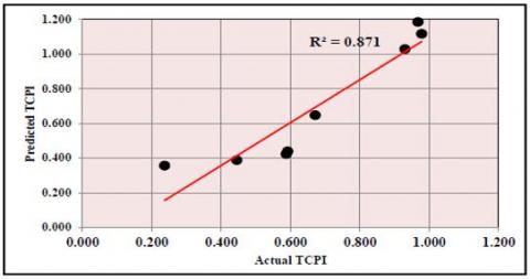
Figure 8. Comparison of Predicted and Actual for TCPI Model
Figure 9. Generalization of TCPI Model
Figure 8 illustrates the predicted values against the actual values for the verification data to show the capacity of the SVM model for TCPI to assess the model. It is clear from this figure that the (R2=87.1%). The results of generalization from the TCPI model with (R2=87.53%) is an excellent as shown in Figure 9.
Mean percentage error (MPE), root mean squared error (RMSE), mean absolute percentage error (MAPE), average accuracy percentage (AA%), coefficient of determination (R2), and coefficient of correlation (R) are the statistical measures most frequently used to assess the model's accuracy [12, 13]. Table 21 clearly shows the comparative study's outputs in terms of results. The average accuracy (AA%) for the CPI, SPI, and TCPI was 96.093%, 91.709%, and 66.024%, respectively, while the correlation coefficients (R) were 92.8%, 98.2%, and 93.3%. As a result, the models' consistency with actual data was very outstanding.
Table 21. The outputs of the validation study for CPI, SPI and TCSPI-SVM models
|
Parameters |
Equations |
|
CPI-SVM Model |
SPI-SVM Model |
TCPI-SVM Model |
|
MPE% |
$\mathrm{MPE}=\left(\frac{\sum \frac{\mathrm{X}-\mathrm{Y}}{\mathrm{X}}}{\mathrm{n}}\right) * 100$ |
(11) |
2.0145 |
0.9071 |
33.6546 |
|
RMSE |
$R M S E=\sqrt{\frac{\sum(Y-X) 2}{n}}$ |
(12) |
0.0969 |
0.0604 |
0.2260 |
|
MAPE% |
$MAPE=\frac{\sum \frac{|\mathrm{X}-\mathrm{Y}|}{\mathrm{X}} * 100 \%}{n}$ |
(13) |
3.907 |
8.291 |
33.976 |
|
AA% |
$(A A \%)=100 \%-M A P E$ |
(14) |
96.093 |
91.709 |
66.024 |
|
R% |
$\mathrm{r}=\frac{\sum(x-\bar{x})(y-\bar{y})}{\sqrt{\sum(x-\bar{x}) 2 \sum(y-\bar{y}) 2}}$ |
(15) |
92.8 |
98.2 |
93.3 |
|
R2% |
86.11 |
96.5 |
87.1 |
||
|
Notes |
|
x=actual value y=estimated value or predicted value n=total number of observations |
|||
Construction oil and gas projects especially Refineries are very important today in Iraq because they help with and support the operation and production process. However, these projects have had significant cost overruns, time overruns, and poor quality, which has hurt their success and is a major concern for the industry, therefore this study's concept came to forecast the earned value indices schedule performance index (SPI), cost performance index (CPI), and to-completion cost performance indicator (TCPI) of implementing projects of refineries using support vector machine. In this study, three models were used, with six variables as inputs which is the BAC, ACWP, BCWP, BCWS, A% and P%. Three equations were found. Many significant findings are shown by the research, including average accuracy (AA%) for the CPI, SPI, and TCPI was 96.093%, 91.709%, and 66.024%, respectively. The correlation coefficients (R) were 92.8%, 98.2%, and 93.3% and the root mean squared error (RMSE) was 0.0969, 0.0604, and 0.2260 respectively. It is noteworthy that the findings of this study serve as a crucial marker and a further prediction guide for forecasting the success of oil projects. The limit of this research is to forecast performance measurement for oil projects, especially refineries. Future studies should concentrate on estimating the performance of different project types utilizing more additional inputs or another artificial methodology like genetic algorithms, dynamic programming, and others.
The corresponding author thanks the Karbala Refinery Project Authority, the general company for oil projects (SCOPE), and the Iraqi Ministry of Oil, for providing us with all the information necessary for the research.
|
SVM |
Support Vector Machine |
|
CPI |
Cost Performance Index |
|
SPI |
Schedule Performance Index |
|
TCPI |
To-Complete Cost Performance Indicator |
|
MPE |
Mean Percentage Error |
|
RMSE |
Root Mean Squared Error |
|
MAPE |
Mean Absolute Percentage Error |
|
AA% |
Average accuracy percentage |
|
R2 |
The Coefficient of Determination |
|
R |
The Coefficient of Correlation |
[1] Kassem, M.A. (2022). Risk management assessment in oil and gas construction projects using structural equation modeling (PLS-SEM). Gases, 2(2): 33-60. https://doi.org/10.3390/gases2020003
[2] AlNoaimi, F.A., Mazzuchi, T.A. (2021). Risk management application in an oil and gas company for projects. International Journal of Business Ethics and Governance, 4(3): 1-30. https://doi.org/10.51325/ijbeg.v4i3.77
[3] Challa, R.K., Rao, K.S. (2022). An effective optimization of time and cost estimation for prefabrication construction management using artificial neural networks. Revue d'Intelligence Artificielle, 36(1): 115-123. https://doi.org/10.18280/ria.360113
[4] Ziyash, A. (2018). Earned value management and its applications: A case of an oil & gas project in Kazakhstan. PM World Journal, 7: 1-23.
[5] Jasim, N.A., Maruf, S.M., Aljumaily, H.S., Al-Zwainy, F. (2020). Predicting index to complete schedule performance indicator in highway projects using artificial neural network model. Archives of Civil Engineering, 66(3): 541-554. http://doi.org/10.24425/ace.2020.134412
[6] Hasan, M.F., Hammody, O., Albayati, K.S. (2022). Estimate final cost of roads using support vector machine. Archives of Civil Engineering, 68(4): 669-682. https://doi.org/10.24425/ace.2022.143061
[7] Juszczyk, M. (2019). On the search of models for early cost estimates of bridges: An SVM-based approach. Buildings, 10(1): 2. https://doi.org/10.3390/buildings10010002
[8] Alawadi, S., Mera, D., Fernández-Delgado, M., Alkhabbas, F., Olsson, C.M., Davidsson, P. (2020). A comparison of machine learning algorithms for forecasting indoor temperature in smart buildings. Energy Systems, 13: 689-705. https://doi.org/10.1007/s12667-020-00376-x
[9] Burhan, A.M., Erzaij, K.R., Hatem, W.A. (2021). Developing a mathematical model for planning repetitive construction projects by using support vector machine technique. Civil and Environmental Engineering, 17(2): 371-379. https://doi.org/10.2478/cee-2021-0039
[10] Eltoukhy, M.G., Nassar, A.H. (2021). Using support vector machine (SVM) for time and cost overrun analysis in construction projects in Egypt. International Journal of Civil Engineering and Technology, 12(3): 5-22. https://doi.org/10.34218/IJCIET.12.3.2021.002
[11] Chandanshive, V.B., Kambekar, A.R. (2021). Prediction of building construction project cost using support vector machine. Industrial Engineering and Strategic Management, 1(1): 31-42. https://doi.org/10.22115/iesm.2021.297399.1015
[12] Susilowati, F., Kurniaji, W.M. (2020). Effective performance evaluation to estimate cost and time using earned value. In IOP Conference Series: Materials Science and Engineering. IOP Publishing, 771(1): 012055. https://doi.org/10.1088/1757-899X/771/1/012055
[13] Hussien, E.A.M., Jasim, N.A. (2021). BIM-Based tool for analysis earned value indicators: Iraq construction projects as a case study. Design Engineering, 130-146. https://www.researchgate.net/publication/352018934