Jehan A. Qahtan![]() | M. S. Hussein*
| M. S. Hussein*![]() | Muhammad Ahsan
| Muhammad Ahsan![]() | Maher Alwuthaynani
| Maher Alwuthaynani![]()
© 2023 IIETA. This article is published by IIETA and is licensed under the CC BY 4.0 license (http://creativecommons.org/licenses/by/4.0/).
OPEN ACCESS
This study delves into the nonlocal inverse boundary-value problem for a second-order, two-dimensional parabolic equation within a rectangular domain. The primary focus is to identify the unknown coefficient and propose a resolution to the problem. The second-order, two-dimensional convection equation is addressed through the direct application of the alternating direction explicit (ADE) finite difference scheme. An adaptation of the ADE scheme is formulated to accommodate mixed boundary conditions, utilizing suitable expressions at the boundaries. Furthermore, unconditional stability is scrutinized through a series of examples. Each ADE scheme typically comprises two substeps, known as upward and downward sweeps, during which values computed at the new time level are incorporated into the discretization template. The inverse problem is restructured into a nonlinear regularized least-square optimization problem, with a defined boundary for the unknown factor, and is effectively resolved using the MATLAB subroutine lsqnonlin from the optimization toolbox. Given the typically ill-posed nature of the problem under investigation, where minor errors in the input data can significantly affect the output, Tikhonov's regularization technique is employed to produce stable and regularized results.
inverse problem, two-dimensional parabolic equation, nonlocal initial conditions, overdetermination condition, (ADE) finite difference schemes, MATLAB, lsqnonlin, Tikhonov technique
In many fields of mathematical modeling, including biology, financial market behavior, medicine, mineral exploration, seismology, seawater desalination, liquid movement in porous media, etc., inverse problems can occur. Numerous authors have studied the two-dimensional heat equation inverse problems in great detail; for instance. In references [1-6], existence and uniqueness of solution have been discussed by many researchers using different methods. While, numerical solutions were also discussed by some researchers as, in reference [7] considered method of fundamental solutions, researchers [8] applied a meshless method. In references [9-16], the Tikhonov regularization was used for solving specific inverse problems. In reference [17], researchers used FDM and predictor corrector method. The two sweeps that make up the ADE scheme are explicit sub steps. When moving from one boundary to another and vice versa, a sweeping step is created. ADM (Explicit or Implicit) is one of the most popular techniques for resolving well-posed one-two dimensions problems. As an illustration, see references [18-22]. Also used in solving in the inverse problems, in references [23, 24]. This method is considered unconditionally stable. By using two different methods of investigation into stability were used, the matrix and the von-Neumann [25, 26]. The inverse problem in this paper has been shown to be uniquely solvable in reference [1]. As no numerical solution has been proposed yet, the main aim of this work is to find such a solution.
The novelty of the current study is to find the solution to the nonlinear nonlocal parabolic equation in two dimensions with a rectangular domain using the ADE scheme with the optimization method.
The paper is structured as follows: the inverse problem's theoretical design in Section 2, while in Section 3, numerical solution which based on Alternating Direction Explicit (ADE) finite difference scheme for direct problem. A numerical method based on a minimization algorithm is presented for solving the inverse problem in Section 4. Present and discuses numerical results in Section 5. Finally, Section 6 presents conclusions.
Consider the inverse problem of retrieving an unknown time-dependent potential coefficient a(τ) in the following two-dimensional parabolic equation:
Zτ(x,y,τ)=c(τ)(Zxx(x,y,τ)+Zyy(x,y,τ))+a(τ)Z(x,y,τ)+F(x,y,τ),(x,y,τ)∈DT (1)
with nonlocal initial condition
Z(x,y,0)+ςZ(x,y,T)=ϕ(x,y),(x,y)∈¯Qx,y (2)
and the homogenous mixed (Neumann, Dirichlet) boundary conditions:
Z(0,y,τ)=Zx(1,y,τ)=0,τ∈[0,T],y∈[0,1] (3)
Zy(x,0,τ)=Z(x,1,τ)=0,τ∈[0,T],x∈[0,1] (4)
and the overdetermination condition:
Z(x0,y0,τ)+∫10∫10 K(x,y)Z(x,y,τ)dydx=μ(τ),0<x0,y0<1,τ∈[0,T] (5)
where, ζ≥0 is known number, 0<ϕ(x,y),μ(τ),c(τ),F(x,y,τ) are given functions, (x0,y0)∈¯Qx,y is some fixed point, a(τ) and Z(x,y,τ) are unknown functions, in the domain DT=ˉQx,y×[0,T], where ¯Qx,y={(x,y):0<y<1,0<x<1}.
The numerical solution of the inverse problem twodimensional parabolic equation (1)-(5) is written as {a(τ),Z(x,y,τ)} such that a(τ)∈C[0,T] and Z(x,y,τ)∈ C2,2,1(DT).
The existences and uniqueness theorems have been proved in reference [5], and mentioned as follows:
2.1 Existence of the inverse problem solution
Assume the following conditions:
E1)
ϕ(x,y),ϕx(x,y),ϕxx(x,y),ϕy(x,y),ϕxy(x,y),ϕyy(x,y)∈C(ˉQx,y),ϕxxy(x,y),ϕxxy(x,y),ϕxxx(x,y),ϕyyy(x,y)∈L2(Qx,y),
ϕ(0,y)=ϕx(1,y)=ϕxx(0,y)=0,y∈[0,1]
ϕy(x,0)=ϕ(x,1)=ϕyy(x,1)=0,x∈[0,1];
E2)
F(x,y,τ),Fx(x,y,τ),Fxx(x,y,τ),Fy(x,y,τ),Fxy(x,y,τ),Fyy(x,y,τ)∈C(DT),Fxxy(x,y,τ),Fxxy(x,y,τ),Fxxx(x,y,τ),Fyyy(x,y,τ)∈L2(DT);
F(0,y,τ)=Fx(1,y,τ)=Fxx(0,y,τ)=0,y∈[0,1],τ∈[0,T]
Fy(x,0,τ)=F(x,1,τ)=Fyy(x,1,τ)=0,x∈[0,1],τ∈[0,T];
E3)
ς≥0, K(x,y)∈L1(Qx,y),0<c(τ)∈C[0,T],μ(τ)∈C1[0,T],μ(τ)≠0,τ∈(0,T].
Theorem 1. Let the assumptions (E1) - (E3) and the condition.
(W3(T)+W4(T))(W1(T)+W2(T)+2)2<1. (6)
where,
W1(T)=3(O1+O2+O3+O4)+3(1+ς)√T(O5+O6+O7+O8).
W2(T)=‖.
W_3(T)=3(1+\varsigma) T.
W_4(T)=\left\|[\mu(\tau)]^{-1}\right\|_{C[0, T]}(1+\varsigma) T O_8.
O_1=\left\|\phi_{x x x}(x, y)\right\|_{L_2\left(Q_{x, y}\right)}, \quad O_2=\left\|\phi_{x y y}(x, y)\right\|_{L_2\left(Q_{x, y}\right)^{\prime}}, \quad O_3=\left\|\phi_{x x y}(x, y)\right\|_{L_2\left(Q_{x, y}\right)},
O_4=\left\|\phi_{y y y}(x, y)\right\|_{L_2\left(Q_{x, y}\right)}, O_5=\left\|\mathcal{F}_{x x x}(x, y, \tau)\right\|_{L_2\left(D_T\right)}, \quad O_6=\left\|\mathcal{F}_{x y y}(x, y, \tau)\right\|_{L_2\left(D_T\right)},
O_4=\left\|\phi_{y y y}(x, y)\right\|_{L_2\left(Q_{x, y}\right)}, O_5=\left\|\mathcal{F}_{x x x}(x, y, \tau)\right\|_{L_2\left(D_T\right)}, \quad O_6=\left\|\mathcal{F}_{x y y}(x, y, \tau)\right\|_{L_2\left(D_T\right)},
O_7=\left\|\mathcal{F}_{x x y}(x, y, \tau)\right\|_{L_2\left(D_T\right)}, \quad O_8=\left\|\mathcal{F}_{y y y}(x, y, \tau)\right\|_{L_2\left(D_T\right)}, \quad O_8=\rho\|c(\tau)\|_{C[0, T]}\left(\sum_{k=1}^{\infty} \sum_{k=1}^{\infty} \lambda_k^{-2}\right)^{\frac{1}{2}}
\lambda_k=\frac{\pi}{2}(2 k-1), \quad k=1,2, \ldots, \quad \rho=1+\int_0^1 \int_0^1|\mathrm{~K}(x, y)| d y d x
be satisfied. Then, the problem (1)-(5) have a single, classical solution in the closed ball K_R of radius R=\left(W_1(T)+\right. W(T)+2) centered at zero in the space E_T^3\left(E_T^3\right. is Banach space).
In the section, we aim to solve the governing equation when the unknown coefficient a(\tau) assumed to be given. That mean we are dealing with a direct problem, and it is require finding the temperature distribution Z(x, y, \tau). In order to handle this problem, we develop ADE scheme which firstly proposed by Barakat and Clark [18], for one-dimensional heat equation. The ADE methodology based on sweeping the spatial axis in a direction of x-space, for example, and then for the opposite direction we sweep in different direction the resulting solution at each sweep direction taken the numerical average in order to maintain the accuracy stability.
We subdivide \mathrm{Q}_{\mathrm{x}, \mathrm{y}} into N_1, N_2 and M subintervals of equal step lengths, form space x=\frac{1}{N_1} and y=\frac{1}{N_2} and time \tau=\frac{T}{M}, where \mathrm{N}_1, \mathrm{~N}_2 and \mathrm{M} are given positive integer. The grid points are given by:
\begin{gathered}x_i=i \Delta x, \quad i=\overline{0, N_1} ; y_j=j \Delta y, \quad j=\overline{0, N_2} . \\ \tau_k=k \Delta \tau, \quad k=\overline{0, M .}\end{gathered}
We denote the discretized form of the quantities as follows;
\begin{aligned} & \mathrm{Z}\left(x_i, y_j, \tau_k\right)=Z_{i, j}^k, a\left(\tau_k\right)=a^k, \mathcal{F}\left(x_i, y_j, \tau_k\right)=\mathcal{F}_{i, j}^k, c\left(\tau_k\right)=c^k, \phi\left(x_i, y_j\right)=\phi_{i, j} \text { and } \mu\left(\tau_k\right)=\mu^k, \\ & \mathrm{~K}\left(x_i, y_j\right)=\mathrm{K}_{i, j}, \text { for } i=\overline{0, N_1}, j=\overline{0, N_2} \text { and } k=\overline{0, M} .\end{aligned}
In this section, the Alternating Direction Explicit Method (ADE) will outline an unconditionally stable numerical procedure for solving the two-dimensional parabolic Eq. (1) with initial condition (2), and boundary conditions (3)-(4) based on the approach described in reference [6]. We will assume that u and v are the solutions of the following equations, which represent the discretization finite differences for (1);
\frac{u_{i, j}^{k+1}-u_{i, j}^k}{\Delta \tau}=c^k\left(\frac{u_{i+1, j}^k-u_{i, j}^k-u_{i, j}^{k+1}+u_{i-1, j}^{k+1}}{(\Delta x)^2}+\frac{u_{i, j+1}^k-u_{i, j}^k-u_{i, j}^{k+1}+u_{i, j-1}^{k+1}}{(\Delta y)^2}\right)+a^k\left(\frac{u_{i, j}^k+u_{i, j}^{k+1}}{2}\right)+\left(\frac{\mathcal{F}_{i, j}^k+\mathcal{F}_{i, j}^{k+1}}{2}\right),
i=\overline{1, N_1}, \quad j=\overline{0, N_2-1} and k=\overline{0, M} (7)
\frac{v_{i, j}^{k+1}-v_{i, j}^k}{\Delta \tau}=c^k\left(\frac{v_{i+1, j}^{k+1}-v_{i, j}^{k+1}-v_{i, j}^k+v_{i-1, j}^k}{(\Delta x)^2}+\frac{v_{i, j+1}^{k+1}-v_{i, j}^{k+1}-v_{i, j}^k+v_{i, j-1}^k}{(\Delta y)^2}\right)+a^k\left(\frac{v_{i, j}^k+v_{i, j}^{k+1}}{2}\right)+\left(\frac{\mathcal{F}_{i, j}^k+\mathcal{F}_{i, j}^{k+1}}{2}\right),
i=\overline{N_1, 1}, \quad j=\overline{N_2-1,0} and k=\overline{0, M} (8)
Simplifying the above equations, we obtain the following explicit difference equations
u_{i, j}^{k+1}=\mathcal{A}^k u_{i, j}^k+\mathcal{B}^k\left(u_{i-1, j}^{k+1}+u_{i+1, j}^k\right)+\mathcal{C}^k\left(u_{i, j-1}^{k+1}+u_{i, j+1}^k\right)+\frac{\Delta \tau}{1+\delta^k}\left(\frac{\mathcal{F}_{i, j}^k+\mathcal{F}_{i, j}^{k+1}}{2}\right),
i=\overline{1, N_1}, \quad j=\overline{0, N_2-1} and k=\overline{0, M} (9)
v_{i, j}^{k+1}=\mathcal{A}^k v_{i, j}^k+\mathcal{B}^k\left(v_{i-1, j}^k+v_{i+1, j}^{k+1}\right)+\mathcal{C}^k\left(v_{i, j-1}^k+v_{i, j+1}^{k+1}\right)+\frac{\Delta \tau}{1+\delta^k}\left(\frac{\mathcal{F}_{i, j}^k+\mathcal{F}_{i, j}^{k+1}}{2}\right),
i=\overline{N_1, 1}, \quad j=\overline{N_2-1,0} and k=\overline{0, M} (10)
where,
\begin{aligned} \mathcal{A}^k & =\left(1-\delta^k\right) /\left(1+\delta^k\right), & k & =\overline{0, M}, \\ \mathcal{B}^k & =\frac{\Delta \tau c^k}{(\Delta x)^2} /\left(1+\delta^k\right), & k & =\overline{0, M}, \\ \mathcal{C}^k & =\frac{\Delta \tau c^k}{(\Delta y)^2} /\left(1+\delta^k\right), & k & =\overline{0, M},\end{aligned}
and
\delta^k=\Delta \tau\left(\frac{c^k}{(\Delta x)^2}+\frac{c^k}{(\Delta y)^2}-\frac{a^k}{2}\right), \quad k=\overline{0, M}.
In order to maintain the stability for Z_{i, j}^k, we use the arithmetic mean of u_{i, j}^k and v_{i, j}^k, specifically as:
\mathrm{Z}_{i, j}^k=\frac{u_{i, j}^k+v_{i, j}^k}{2} (11)
Furthermore, assume \varsigma=0 for simplicity (although it is possible to select a value other than zero, doing so will require data optimization, and the program is already built into the performance optimization, so the calculations will take a long time), and let the boundary and initial conditions are satisfied byv_{i, j}^k and u_{i, j}^k, then FDM discretizes Eqs. (2)-(4) as
u_{i, j}^0=v_{i, j}^0=\phi_{i, j}, \quad i=\overline{0, N_1}, \quad j=\overline{0, N_2} (12)
u_{0, j}^k=v_{0, j}^k=0, \quad u_{N_1+1, j}^k=u_{N_1, j}^k, \quad v_{N_1+1, j}^k=v_{N_1, j}^k, \quad k=\overline{0, M}, \quad j=\overline{0, N_2} (13)
u_{i, 0}^k=u_{i,-1}^k, \quad v_{i, 0}^k=v_{i,-1}^k, \quad u_{i, N_2}^k=v_{i, N_2}^k=0, \quad k=\overline{0, M}, \quad i=\overline{0, N_1} (14)
The doable integral overdetermination condition (5) is finally discretized by the trapezoidal rule as:
\begin{gathered}\mu\left(\tau_k\right)=Z_{i_0, j_0}^k+\frac{1}{4 N_1 N_2}\left(K_{0,0} Z_{0,0}^k+K_{N_1, 0} Z_{N_1, 0}^k+K_{0, N_2} Z_{0, N_2}^k+K_{N_1, N_2} Z_{N_1, N_2}^k+2 \sum_{i=1}^{N_1-1} K_{i, 0} Z_{i, 0}^k+2 \sum_{i=1}^{N_1-1} K_{i, N_2} Z_{i, N_2}^k+2 \sum_{j=1}^{N_2-1} K_{0, j} Z_{0, j}^k\right. \\ \left.+2 \sum_{j=1}^{N_2-1} K_{N_1, j} Z_{N_1, j}^k+4 \sum_{j=1}^{N_2-1} \sum_{i=1}^{N_1-1} K_{i, j} Z_{i, j}^k\right), k=\overline{0, M}\end{gathered} (15)
3.1 Boundary treatment
Since there are points out of the domain such as u_{N_1+1, j}^k, v_{N_1+1, j}^k, u_{i,-1}^k and v_{i,-1}^k, when i=N_1 and j=0 respectively, which are located out of domain values that can be calculated directly from boundary conditions. We noticed when using the central, backward, or three-point scheme to approximate Eqs. (3)-(4), it appears points will also be out of domain, so we use the forward finite difference scheme to approximate Eqs. (3)-(4), then we get:
u_{N_1+1,0}^k=u_{N_1, 0}^k, \quad v_{N_1+1,0}^k=v_{N_1, 0}^k, \quad k=\overline{0, M},
u_{i,-1}^k=u_{i, 0}^k, \quad v_{i,-1}^k=v_{i, 0}^k, \quad k=\overline{0, M}.
After substituting into Eqs. (9)-(10), we get as:
u_{i, 0}^{k+1}=\mathcal{A}^k u_{i, 0}^k+\mathcal{B}^k\left(u_{i-1,0}^{k+1}+u_{i+1,0}^k\right)+\mathcal{C}^k\left(u_{i, 0}^{k+1}+u_{i, 1}^k\right)+\frac{\Delta \tau}{2\left(1+\delta^k\right)}\left(\mathcal{F}_{i, 0}^k+\mathcal{F}_{i, 0}^{k+1}\right), \quad k=\overline{0, M} and i=\overline{1, N_1-1}
simplifying the above equations, we get:
u_{i, 0}^{k+1}=\left(\frac{1}{1-\mathcal{C}^k}\right)\left(\mathcal{A}^k u_{i, 0}^k+\mathcal{B}^k\left(u_{i-1,0}^{k+1}+u_{i+1,0}^k\right)+\mathcal{C}^k u_{i, 1}^k+\frac{\Delta \tau}{2\left(1+\delta^k\right)}\left(\mathcal{F}_{i, 0}^k+\mathcal{F}_{i, 0}^{k+1}\right)\right), \quad k=\overline{0, M} and i=\overline{1, N_1-1} (16)
With similar steps, we can process the rest of the points:
u_{N_1, 0}^{k+1}=\left(\frac{1}{1-\mathcal{C}^k}\right)\left(\mathcal{A}^k u_{N_1, 0}^k+\mathcal{B}^k\left(u_{N_1-1,0}^{k+1}+u_{N_1, 0}^k\right)+\mathcal{C}^k u_{N_1, 1}^k+\frac{\Delta \tau}{2\left(1+\delta^k\right)}\left(\mathcal{F}_{N_1, 0}^k+\mathcal{F}_{N_1, 0}^{k+1}\right)\right), \quad k=\overline{0, M} (17)
u_{N_1, j}^{k+1}=\mathcal{A}^k u_{N_1, j}^k+\mathcal{B}^k\left(u_{N_1-1, j}^{k+1}+u_{N_1, j}^k\right)+\mathcal{C}^k\left(u_{N_1, j-1}^{k+1}+u_{N_1, j+1}^k\right)+\frac{\Delta \tau}{2\left(1+\delta^k\right)}\left(\mathcal{F}_{N_1, j}^k+\mathcal{F}_{N_1, j}^{k+1}\right), k=\overline{0, M} and j=\overline{1, N_2-1} (18)
v_{N_1, j}^{k+1}=\left(\frac{1}{1-\mathcal{B}^k}\right)\left(\mathcal{A}^k v_{N_1, j}^k+\mathcal{B}^k v_{N_1-1, j}^k+\mathcal{C}^k\left(v_{N_1, j-1}^k+v_{N_1, j+1}^{k+1}\right)+\frac{\Delta \tau}{2\left(1+\delta^k\right)}\left(\mathcal{F}_{N_1, j}^k+\mathcal{F}_{N_1, j}^{k+1}\right)\right), k=\overline{0, M}, j=\overline{N_2-1,1} (19)
v_{N_1, 0}^{k+1}=\left(\frac{1}{1-\mathcal{B}^k}\right)\left(\mathcal{A}^k v_{N_1, 0}^k+\mathcal{B}^k v_{N_1-1,0}^k+\mathcal{C}^k\left(v_{N_1, 0}^k+v_{N_1, 1}^{k+1}\right)+\frac{\Delta \tau}{1+\delta^k}\left(\frac{\mathcal{F}_{N_1, 0}^k+\mathcal{F}_{N_1, 0}^{k+1}}{2}\right)\right), \quad k=\overline{0, M} (20)
v_{i, 0}^{k+1}=\mathcal{A}^k v_{i, 0}^k+\mathcal{B}^k\left(v_{i-1,0}^k+v_{i+1,0}^{k+1}\right)+\mathcal{C}^k\left(v_{i, 0}^k+v_{i, 1}^{k+1}\right)+\frac{\Delta \tau}{1+\delta^k}\left(\frac{\mathcal{F}_{i, 0}^k+\mathcal{F}_{i, 0}^{k+1}}{2}\right), \quad k=\overline{0, M} and i=\overline{N_1-1,1} (21)
3.2 Example for direct problem
We take T=1 in all examples, for simplicity.
Example 1:
In the first stage, we assume the situation where the unidentified coefficients are provided in order to test the effectiveness of the proposed ADE scheme for direct problems. We have the precise solution as
\mathrm{Z}(x, y, \tau)=\frac{e^{-\tau} \cos \left(\frac{y \pi}{2}\right) \sin \left(\frac{x \pi}{2}\right)}{150}, \quad(x, y, \tau) \in D_T
and the input data are as follows:
\mathrm{K}(x, y)=x y, \quad \phi(x, y)=\frac{\cos \left(\frac{y \pi}{2}\right) \sin \left(\frac{x \pi}{2}\right)}{150}, \quad(x, y) \in \overline{\mathrm{Q}}_{x, y}
c(\tau)=\frac{(1.1-\tau)}{1000}, \quad a(\tau)=\frac{(\tau-12)}{5}, \quad \mathrm{Z}(0.5,0.5, \tau)=0.003333 e^{-\tau}, \quad \tau \in[0,1]
\mu(\tau)=\mathrm{Z}(0.5,0.5, \tau)+\frac{4(-2+\pi)}{75 \pi^4} e^{-\tau}, \quad \tau \in[0,1]
f(x, y, \tau)=(0.0093695-0.001366 \tau) e^{-\tau} \cos \left(\frac{y \pi}{2}\right) \sin \left(\frac{x \pi}{2}\right), \quad(x, y, \tau) \in D_T
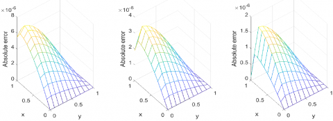
Figure 1. The graphs showing absolute errors for the direct problem (17)-(18), when sizes of mesh N_1=N_2=10 and M \in \{20,40,80\}
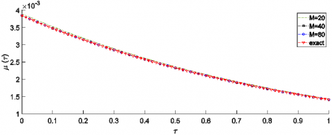
Figure 2. The numerical value and accurate for \mu(\tau), when sizes of mesh \mathrm{N}_1=\mathrm{N}_2=10, and M \in\{20,40,80\}
The absolute error diagram for interior points when sizes of mesh for the space is \mathrm{N}_1=\mathrm{N}_2=10, and time mesh are taken as 20, 40, and 80 is shown in Figure 1. This graph demonstrates the achievement of mesh independence, numerical solutions for each time mesh selection converge to an exact solution, and high agreement are obtained. Figures 1 and 2 illustrate how the results become more precise and clearly converge as the number of discretization's increases.
We aim to find numerical solutions to nonlinear inverse problems (1)-(5) that mean a(\tau) is unknown potential coefficient. As the inverse problem is being solved iteratively, we considered a(0) as a constant initial guess. This value can be obtained by using the input data at initial time \tau=0, which will be handled in next subsection. We recast this type of problem as a nonlinear minimization problem. In other words, we try to minimize the difference between the measured data \mu(\tau) and the numerically computed solution (15). Because the problem is ill-posed, so we use Tikhonov's regularization method to find a stable numerical solution. From condition (5), the Tikhonov's regularization functional can be imposed as follows:
F(a)=\left\|\mathrm{Z}\left(x_0, y_0, \tau\right)+\int_0^1 \int_0^1 \mathrm{~K}(x, y) \mathrm{Z}(x, y, \tau) d y d x-\mu(\tau)\right\|_{L^2[0, T]}^2+\beta\|a(\tau)\|^2 (22)
where, \beta \geq 0, is a regularization parameter should be determined according to some selections methods like L-curve method by Hansen and O'Leary [27], Morozov's discrepancy principle [28]. We used trial and error, in our work as described in reference [29]. The discretization of (22) is as;
F(\underline{a})=\sum_{j=1}^N\left[\mathrm{Z}\left(x_0, y_0, \tau_j\right)+\int_0^1 \int_0^1 \mathrm{~K}(x, y) \mathrm{Z}\left(x, y, \tau_j\right) d y d x-\mu\left(\tau_j\right)\right]^2+\beta \sum_{j=1}^N a_j^2 (23)
The unregularized case, i.e., β = 0, produces the regular nonlinear least-squares functional, which is inherently unstable when dealing with noisy data. The toolbox subroutine lsqnonlin from MATLAB is used to minimize the functional F, which does not need the user to provide the gradient of the objective functional (23). The lsqnonlin subroutine performs a constrained nonlinear optimization in order to find the minimum of a scalar function with numerous variables. We use the following parameters for the subroutine:
The solution to the inverse problem (1)-(5) is investigated to both noisy and exact measurements (5).
A numerically simulated of the noisy data is adding by a random error as follows:
\mu^\epsilon\left(\tau_j\right)=\mu\left(\tau_j\right)+\epsilon_j, \quad j=\overline{0, M} (24)
where, \epsilon, is random Gaussian normal distribution vectors with standard deviations σ and mean equal to zero, such that
\sigma=p \times \max _{\tau \in[0, T]}|\mu(\tau)| (25)
where, p is the percentage of noise. We use the MATLAB bulletin function normrnd as follows:
\underline{\epsilon}=\operatorname{normrnd}(0, \sigma, M) (26)
To generate the random variables \underline{\epsilon}=\left(\epsilon_j\right) and j=\overline{0, M}.
4.1 Initial guess
As mentioned before, we require an initial guess to begin with when solving the inverse problem iteratively. These values a(0) can be calculated using the following input data:
Consider the nonlinear inverse problem (1)-(5) with an unknown potential coefficient a(τ) evaluate, the nonlocal overdetermination condition (5) at \tau=0, and we have after differentiating with respect to time:
\mathrm{Z}\left(x_0, y_0, \tau\right)+\int_0^1 \int_0^1 \mathrm{~K}(x, y) \mathrm{Z}(x, y, \tau) d y d x=\mu(\tau), \int_0^1 \int_0^1 K(x, y) \mathrm{Z}_\tau(x, y, \tau) d y d x=\mu^{\prime}(\tau)-\mathrm{Z}_\tau\left(x_0, y_0, \tau\right) (27)
multiplying Eq. (1) by K(x,y) and integrating twice with respect to x and y over the interval [0, 1], we have:
\int_0^1 \int_0^1 K(x, y) \mathrm{Z}_\tau(x, y, \tau) d y d x=c(\tau) \int_0^1 \int_0^1 K(x, y)\left(\mathrm{Z}_{x x}(x, y, \tau)+\mathrm{Z}_{y y}(x, y, \tau)\right) d y d x
+a(\tau) \int_0^1 \int_0^1 K(x, y) \mathrm{Z}(x, y, \tau) d y d x+\int_0^1 \int_0^1 K(x, y) \mathcal{F}(x, y, \tau) d y d x (28)
evaluating the Eq. (28) at \tau=0, we get:
\mu^{\prime}(0)-\phi^{\prime}\left(x_0, y_0\right)=g_1+a(0)\left(\mu(0)-\phi\left(x_0, y_0\right)\right)+g_2 (29)
The first guess was made using Eqs. (2) and (29).
a(0)=\frac{\mu^{\prime}(0)-\phi^{\prime}\left(x_0, y_0\right)-g_1-g_2}{\mu(0)-\phi\left(x_0, y_0\right)} (30)
where,
g_1=c(0) \int_0^1 \int_0^1 K(x, y)\left(\phi_{x x}(x, y)+\phi_{y y}(x, y)\right) d y d x,
g_2=\int_0^1 \int_0^1 K(x, y) \mathcal{F}(x, y, 0) d y d x.
provided that \mu(0)-\phi\left(x_0, y_0\right) did not vanish.
The root mean squares errors (RMSE) utilized, calculated to determine the accuracy of the specified coefficient.
\operatorname{rmse}(a)=\sqrt{\frac{1}{M} \sum_{i=1}^M\left(a_i^{\text {exact }}-a_i^{\text {numerical }}\right)^2} (31)
For simplicity, we fix spatial mesh to be N_1=N_2=10 and time mesh to be \mathrm{M}=40 which was discovered to be sufficiently accurate to ensure that any finer mesh as N_1=N_2=20 and M=80, had no effect on the numerical solution's stability or accuracy.
Next, we consider a numerical experiment for the twodimensional parabolic inverse problem (1)-(5) with the same input data in example 1 except the coefficient a(\tau) is unknown. The initial guess was taken a_0=-2.4 given by Eq. (30). It is easy to verify that the input data verify the conditions El-E3 and Eq. (6), hence the inverse two-dimensional parabolic problem (1)-(5) has a unique solution.
Case 1: No regularization and no noise
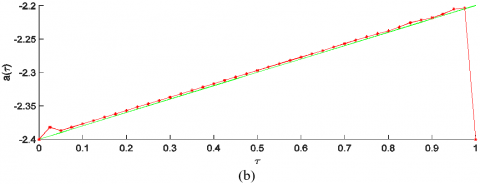
The ideal numerical solution is discussed when, p=0 i.e., no noise included in Eq. (25). The objective function (23) represented Figure 3 (a), and a speed declining convergence is seen for achieving a shorter order tolerance O\left(10^{-12}\right) in just below 5 iterations. Figure 3 (b) shows numerical results for a(\tau). The stability of the approximation has been tested using inclusion of perturbed data.
Case 2: No regularization and with noise
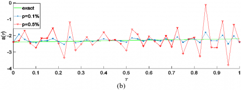
In this case, we perturb the measured data with p \in \{0.1,0.5\} \% noise added as in Eq. (25). In the absence of regularization, Figure 4 displays the related numerical outcomes. From Figure 4 (a) the criterion yields the iteration number =5, revealing that the objective function minimization (23) has converged to small stationary values of orders \mathrm{O} \left(10^{-7}\right) and \mathrm{O}\left(10^{-8}\right). As seen in Figure 4(b), the numerical solution of \mathrm{a}(\tau). Diverges from the exact solution but remains on the same path when the value of additive noise increases in Eq. (25).
Case 3: With noise and Tikhonov’s regularization
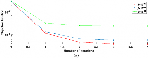
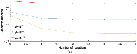
To restore the stability some regularization should be applied. To replicate real input data, noise of p \in\{0.1,0.5\} \% is included with regularization \beta \in\left\{0,10^{-12}, \ldots, 10^{-7}\right\}. Figure 5 (a) and Figure 6 (a), the criterion yields the iteration number =4, revealing that the objective function minimization (23). Figure 5 (b) and Figure 6 (b), show the potential unknown coefficient \mathrm{a}(\tau). These Figures show that results are almost completely smooth, especially in the range [0,0.8], before instabilities begin to show up when noise levels increase from 0.1 \% to 0.5 \%. A very excellent agreement is established while there is \beta=10^{-12}, and \beta=10^{-8} respectively. Moreover, Table 1 is associated \operatorname{rmse}(a) values show that a reasonable range of values can be seen, with the best retrieval occurs at the smallest rmse (a). See the numerical results in Table 1 and Figures 5-6 for more information.
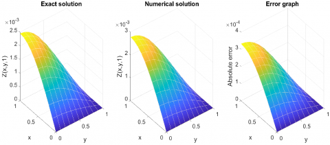
The numerical and exact temperatures Z(x, y, \tau), with p= 0.1 \% noise, \beta=10^{-12}, \mathrm{p}=0.5 \% noise, \beta=10^{-8}, as well as the absolute error between them are illustrated in Figures 7 and 8.
Table 1. The r m s e(a) (31) for the regularization \beta \in\left\{0,10^{-12}, \ldots, 10^{-7}\right\} and noise p \in\{0.1,0.5\} \%
|
β |
0 |
10-12 |
10-11 |
10-10 |
10-9 |
10-8 |
10-7 |
|
|
p=0.1% |
rmse(a) |
0.1572 |
0.1565 |
0.2576 |
0.3723 |
0.3835 |
0.4854 |
0.7381 |
|
p=0.5% |
rmse(a) |
0.6683 |
0.6671 |
0.6803 |
0.6788 |
0.4927 |
0.4916 |
0.7366 |
Figure 3. (a) Objective function (23) and (b) a(τ) with noise free and without regularization
Figure 4. (a) Objective function (23) and (b) Reconstruction of a(τ), for different noise level p \in\{0.1,0.5\} \% and no regularization
Figure 5. (a) Objective function (23) and (b) a(τ), for \beta=\left\{10^{-12}, 10^{-11}, 10^{-10}\right\} and p=0.1 \% noise
Figure 6. (a) Objective function (23) and (b) a(τ), for \beta=\left\{10^{-10}, 10^{-9}, 10^{-8}\right\} and p=0.5 \% noise
Figure 7. Both accurate and numerical Z(x, y, \tau), with p=0.1 \% noise, and \beta=10^{-12}, as well as the absolute error between them
Figure 8. both accurate and numerical Z(x, y, \tau), with p=0.5 \% noise and \beta=10^{-8}, as well as the absolute error between them
The second order, two-dimensional convection equation with time-dependent prospective coefficient a(\tau) under over specified condition of general integral type. The ADE finite difference schemes, in conjunction with the trapezoidal rule quadrature has been used for direct problems. The instability brought on by the ill-posed problem was resolved using the Tikhonov regularization. The RMS values for noise p=0 and \beta=0 were contrasted for the numerical test problem. It has been noted that a stable solution that is accurate with p= 0.1 \% and p=0.5 \% noise is produced upon the introduction of regularization with \beta=10^{-12} to 10^{-7}, and with \beta= 10^{-10} to 10^{-7} respectively. We suggest the following future work is possible, the use of numerical methods different from the methods used in this thesis as shifted Chebyshev tau, predictor-corrector and a meshless to solve the direct problems.
|
F |
Nonlinear objective least-squares functions |
|
lsqnonlin |
MATLAB optimization routine |
|
normrnd |
MATLAB function generating Gaussian random numbers |
|
βi |
Regularization parameter |
|
ϵ |
Total amount of noise |
|
p |
Percentage of noise |
|
rmse |
Root mean square equation |
[1] Azizbayov, E.I., Mehraliyev, Y.T. (2020). Nonlocal inverse boundary-value problem for a 2D parabolic equation with integral overdetermination condition. Carpathian Mathematical Publications, 12(1): 23-33. https://doi.org/10.15330/cmp.12.1.23-33
[2] Anwer, F., Hussein, M.S. (2022). Retrieval of timewise coefficients in the Heat Equation from nonlocal overdetermination conditions. Iraqi Journal of Science, 63(3): 1184-1199. https://doi.org/10.24996/ijs.2022.63.3.24
[3] Kinash, N.Y. (2018). A nonlocal inverse problem for the two-dimensional Heat-Conduction Equation. Journal of Mathematical Sciences, 231(4): 558-572.
[4] Kumar, P., Mohan, M.T. (2022). Existence, uniqueness and stability of an inverse problem for two-dimensional convective Brinkman-Forchheimer equations with the integral overdetermination. Banach Journal of Mathematical Analysis, 16(4): 58. https://doi.org/10.1007/s43037-022-00213-6
[5] Nachman, A.I. (1996). Global uniqueness for a two-dimensional inverse boundary value problem. Annals of Mathematics, 71-96. https://doi.org/10.2307/2118653
[6] Sazaklioglu, A.U., Ashyralyev, A., Erdogan, A.S. (2017). Existence and uniqueness results for an inverse problem for semilinear parabolic equations. Filomat, 31(4): 1057-1064. https://www.jstor.org/stable/24902204
[7] Johansson, B.T., Lesnic, D., Reeve, T. (2011). A method of fundamental solutions for two-dimensional heat conduction. International Journal of Computer Mathematics, 88(8): 1697-1713. https://doi.org/10.1080/00207160.2010.522233
[8] Dawson, M., Borman, D., Hammond, R.B., Lesnic, D., Rhodes, D. (2013). A meshless method for solving a two‐dimensional transient inverse geometric problem. International Journal of Numerical Methods for Heat & Fluid Flow, 23(5): 790-817. https://doi.org/10.1108/HFF-08-2011-0153
[9] Hussein, M.S., Lesnic, D. (2015). Identification of the time-dependent conductivity of an inhomogeneous diffusive material. Applied Mathematics and Computation, 269: 35-58. https://doi.org/10.1016/j.amc.2015.07.039
[10] Hussein, M.S., Lesnic, D. (2016). Simultaneous determination of time and space-dependent coefficients in a parabolic equation. Communications in Nonlinear Science and Numerical Simulation, 33: 194-217. https://doi.org/10.1016/j.cnsns.2015.09.008
[11] Huntul, M.J., Hussein, M.S. (2021). Simultaneous identification of thermal conductivity and heat source in the Heat Equation. Iraqi Journal of Science, 62(6): 1968-1978. https://doi.org/10.24996/ijs.2021.62.6.22
[12] Hussein, M.S., Adil, Z. (2020). Numerical solution for two-sided Stefan problem. Iraqi Journal of Science, 61(2): 444-452. https://doi.org/10.24996/ijs.2020.61.2.24
[13] Qassim, M., Hussein, M.S. (2021). Numerical solution to recover time-dependent coefficient and free boundary from nonlocal and Stefan type overdetermination conditions in Heat Equation. Iraqi Journal of Science, 62(3): 950-960. https://doi.org/10.24996/ijs.2021.62.3.25
[14] Mehraliyev, Y.T., Ramazanova, A.T., Huntul, M.J. (2022). An inverse boundary value problem for a two-dimensional pseudo-parabolic equation of third order. Results in Applied Mathematics, 14: 100274. https://doi.org/10.1016/j.rinam.2022.100274
[15] Qahtan, J. A., Hussein, M. (2023). Reconstruction of timewise dependent coefficient and free boundary in nonlocal diffusion equation with Stefan and heat flux as overdetermination conditions. Iraqi Journal of Science, 64(5): 2449-2465. https://doi.org/10.24996/ijs.2023.64.5.30
[16] Ibraheem, Q.W., Hussein, M.S. (2023). Determination of time-dependent coefficient in time fractional heat equation. Partial Differential Equations in Applied Mathematics, 7: 100492. https://doi.org/10.1016/j.padiff.2023.100492
[17] Kanca, F., Baglan, I. (2021). Analysis for two-dimensional inverse quasilinear parabolic problem by Fourier method. Inverse Problems in Science and Engineering, 29(12): 1912-1945. https://doi.org/10.1080/17415977.2021.1890068
[18] Barakat, H.Z., Clark, J.A. (1966). On the solution of the diffusion equations by numerical methods. Journal of Heat Transfer, 88(4): 421-427. https://doi.org/10.1115/1.3691590
[19] Bučková, Z., Pólvora, P., Ehrhardt, M., Günther, M. (2016). Implementation of alternating direction explicit methods for higher dimensional Black-Scholes equations. In AIP Conference Proceedings. AIP Publishing LLC, 1773(1): 030001. https://doi.org/10.1063/1.4964961
[20] Leung, S., Osher, S. (2005). An alternating direction explicit (ADE) scheme for time-dependent evolution equations. Preprint UCLA June, 9, 2005.
[21] Pealat, G., Duffy, D.J. (2011). The alternating direction explicit (ADE) method for one‐factor problems. Wilmott, 2011(54): 54-60. https://doi.org/10.1002/wilm.10014
[22] Prassetyo, S.H., Gutierrez, M. (2018). High‐order ADE scheme for solving the fluid diffusion equation in non‐uniform grids and its application in coupled hydro‐mechanical simulation. International Journal for Numerical and Analytical Methods in Geomechanics, 42(16): 1976-2000. https://doi.org/10.1002/nag.2843
[23] Huntul, M.J., Lesnic, D. (2019). Determination of a time-dependent free boundary in a two-dimensional parabolic problem. International Journal of Applied and Computational Mathematics, 5(4): 118. https://doi.org/10.1007/s40819-019-0700-5
[24] Hussein, M.S., Lesnic, D., Johansson, B.T., Hazanee, A. (2018). Identification of a multi-dimensional space-dependent heat source from boundary data. Applied Mathematical Modelling, 54: 202-220. https://doi.org/10.1016/j.apm.2017.09.029
[25] Buckova, Z., Ehrhardt, M., Günther, M. (2015). Alternating direction explicit methods for convection diffusion equations. Acta Mathematica Universitatis Comenianae, 84(2): 309-325.
[26] Campbell, L.J., Yin, B. (2007). On the stability of alternating‐direction explicit methods for advection‐diffusion equations. Numerical Methods for Partial Differential Equations: An International Journal, 23(6): 1429-1444. https://doi.org/10.1002/num.20233
[27] Hansen, P.C., O’Leary, D.P. (1993). The use of the L-curve in the regularization of discrete ill-posed problems. SIAM Journal on Scientific Computing, 14(6): 1487-1503. https://doi.org/10.1137/0914086
[28] Bonesky, T. (2008). Morozov's discrepancy principle and Tikhonov-type functionals. Inverse Problems, 25(1): 015015. https://doi.org/10.1088/0266-5611/25/1/015015
[29] Dennis, B.H., Dulikravich, G.S., Yoshimura, S. (2004). A finite element formulation for the determination of unknown boundary conditions for three-dimensional steady thermoelastic problems. Journal of Heat Transfer, 126(1): 110-118. https://doi.org/10.1115/1.1640360