Danielle Khalife*![]() | Jad Yammine
| Jad Yammine![]() | Sanabel Rahal
| Sanabel Rahal![]() | Sibelle Freiha
| Sibelle Freiha![]()
© 2023 IIETA. This article is published by IIETA and is licensed under the CC BY 4.0 license (http://creativecommons.org/licenses/by/4.0/).
OPEN ACCESS
The computation of fair values for exotic options often necessitates complex pricing techniques, which remain sparsely addressed in academic literature. Predominantly, the assessment of fair value for vanilla options relies on methodologies such as the Black-Scholes model or Monte Carlo simulations. This study proposes an innovative, dynamic approach to pricing, leveraging artificial intelligence in conjunction with the Heston model and a Monte Carlo simulation engine. This approach aims to furnish estimates of the prices for Barrier and Asian options. To enhance the accuracy of the model, calibration was performed employing a supervised machine learning algorithm, a continuous risk-free curve, and a dynamic implied volatility surface, derived from the current market data of vanilla options on S&P 500 futures. The amalgamation of these models yields instantaneous pricing for exotic option derivatives, contingent on the investor's determination of time to maturity and barrier levels. The efficacy of the model was evaluated by comparing the output prices to theoretical model predictions and a selection of over-the-counter traded options. Our findings indicate that the proposed dynamic, integrated approach substantially reduces the disparity between the theoretical models and current market prices. The prices calculated by our model demonstrate a marginal error of merely 0.33% in comparison to market prices, a significant improvement over the considerably larger error of 3.12% exhibited by traditional models.
exotic options, artificial intelligence, Heston model, Monte Carlo simulation, calibration, strike price, vanilla options, implied volatility
1.1 General background of the topic
Banks and other financial institutions widely employ mathematical models in their efforts to price and value financial derivatives. Despite the persistent use of the Black-Scholes model for option pricing and valuation by industry professionals, a significant body of empirical research suggests that this model inadequately captures the dynamics of the underlying asset price process. The Black-Scholes model assumes that the underlying asset follows a geometric Brownian motion with constant volatility. However, the options market pricing typically implies different volatilities for varying strike prices and maturities. As a consequence of this limitation, the Black-Scholes model is often subject to substantial pricing and hedging discrepancies.
1.2 Problem statement
Liu and Wang [1] sought to merge artificial intelligence and mathematical models, employing an innovative approach that integrated Black-Scholes autoregression with deep learning. The application of autoregression, which predicts future trends based on historical data, demonstrated promise. However, given the temporal variations in historical volatility and time to maturity, further research is necessary to fully realize these initial observations. In efforts to mitigate the specification error inherent to the Black-Scholes model, several alternative models have been proposed that relax some of its unrealistic assumptions. These extended models are broadly categorized into single-factor models, which include deterministic volatility function models and constant elasticity of variance models, and multi-factor models, such as Merton's [2] and Bates' [3] jump-diffusion models, as well as the stochastic volatility models of Hull and White [4] and Heston [5].
The Heston model, a financial framework that emphasizes evolving volatility, is particularly significant in the context of precise option pricing. 'Plain vanilla' options, being the most fundamental type, grant the holder the right to purchase or sell an asset at an agreed price and time. However, 'exotic' options, which are more complex, feature unique characteristics that allow for greater customization. To predict outcomes in scenarios characterized by substantial uncertainty, the Monte Carlo simulation, a tool for probability modeling, is frequently employed in options pricing.
Model risk emerges as a predominant concern, given the high dependence of exotic option prices on the efficiency of the deployed model, and the fact that each model relaxes certain Black-Scholes assumptions. Despite these models exhibiting improved accuracy, the model risk to which market participants are exposed persists. The challenge that therefore necessitates examination is whether this risk could be minimized through the deployment of a more intricate and dynamic alternative approach.
1.3 Significance of the study
This study is centered on the development of an AI-based model designed to account for market sensitivity in the pricing and hedging of exotic options, such as Barrier and Asian options. Diverging from prior research, our empirical investigation endeavors to fit the model to observable liquid options and evaluate its proficiency in hedging exotic options. Consideration is also given to the calibration of models by practitioners based on market data, facilitating accurate computation of model risk. The outcomes of this study are anticipated to equip investors with a comprehensive tool for pricing exotic options and ensuring market fairness, offering valuable insights to practitioners, regulators, and academics in the fields of finance and mathematics.
The initial dataset employed in our model, consisting of S&P 500 vanilla call option prices, was procured through machine learning techniques. Aiming to curtail error in the pricing process, the price was determined through the fusion of two models — the Heston model and the Monte Carlo simulation — into a singular model, predicated on machine learning techniques. To simplify the pricing process, the output from the Heston model was utilized as input data for the Monte Carlo simulation model. This methodology was subsequently applied and tested on three forms of prevalent exotic options: Asian options, Up-and-Out barrier options, and Down-and-Out barrier options.
Model parameters are derived through a calibration process, the objective of which is to minimize the discrepancy between the extracted prices of vanilla options for the S&P 500 and the prices calculated by the Heston model for the precise parameters of the extracted data. In the subsequent time step, these model parameters are incorporated into a Monte Carlo pricing model for the pricing of Barrier and Asian options. This procedure is repeated until the maturity of the exotic options. To assess the accuracy of the devised model, a sample of 34 randomly selected over-the-counter (OTC) options, priced by an international market maker employing undisclosed methods, was collected for comparison with the results from the developed dynamic model. The output prices generated by the developed model were also juxtaposed with the theoretical prices ascertained by models including Black-Scholes and the Trinomial models. The intention behind such a comparison was to ascertain whether a dynamic approach yield results closer to current OTC prices than traditional approaches.
This study aspires to bridge the previously identified gap between current OTC prices and theoretical model prices. Machine learning is employed to determine the appropriate model parameter values and to amalgamate different models into a single, reliable pricing process. The rationale behind this approach is its potential contribution to ongoing research endeavours seeking to enhance the fair valuation of such complex yet highly sought-after financial derivative products. Since the inception of the Black-Scholes model (1973), the mechanism of pricing options has remained relatively simple and expedient, largely due to the model's assumption of constant values for both the risk-free rate and volatility. To enhance the congruence between predicted and actual option values, Heston [5] introduced a mathematical model wherein volatility is treated as a stochastic random variable.
1.4 Applications of machine learning and neural networks in option pricing
A radical transformation has been ushered in the pricing mechanics of options products, enabled by the advent of Machine Learning (ML) which leverages the principle of super-human intelligence via neural networks [6, 7] and the concept of Big Data, thereby birthing a new field of analytics. Neural networks were initially deployed in vanilla pricing through stochastic volatility models by McGhee [8] and Horvath et al. [9]. Notably, contracts pertaining to exotic option pricing were predominantly path-independent, with a few exceptions [10]. Nonetheless, the notion of acceleration assumes significance in the context of calibration, particularly in instances of inadequate solutions such as stochastic alpha beta rho in AI applications.
Hutchinson et al. [11] were the pioneers in applying ML to option pricing, where they discerned the distribution algorithm underlying options price fluctuations. The system employed neural networks, demonstrating exceptional proficiency in estimating options’ prices. The homogeneity hint, later managed by Kakkad et al. [12], was originally introduced by Dugas et al. [13] to restrict the range of potential outcomes. This hint took into account the uniformity of the option pricing function in strike and asset prices. Subsequently, Hahn [14] implemented ML in the Australian equity options market with an addendum: a specific volatility model was proposed and constructed based on short- and long-term historical volatility, ANN-based volatility, and the GARCH-based volatility model. This model was associated with the extant stochastic model. In the same year, Audrino and Colangelo [15] applied ML in a novel semi-parametric approach for implicit volatility surface, decreasing the residuals between predicted and theoretical implied volatility.
Another application of ML in option pricing was observed in the work of Kakkad et al. [12], who developed a hybrid model as a fusion of various option pricing models (Monte Carlo, BS, SVR). Kakkad et al. [12] introduced two novelties: the bank nifty and the uniformity hint. The bank nifty, notably, is traded on the National Stock Exchange of India Limited (NSE). On a different note, neural networks were utilized by Fang and George [16] in a successful effort to correlate the prices of an Asian option and a closed-form model. Two stimulating experiments were conducted, yielding conclusive results regarding the significant enhancement of the closed-form model's performance. De Spiegeleer, Madan, Reyners, and Schoutens applied the Gaussian Process Regression model to predict the prices of European options [10], and subsequently, used this model for the alternative purpose of calculating the implied volatility surface.
The outcomes of these neural network advancements have been categorized into three classifications by Mezofi and Szabo [17]. The first encompasses the prediction of implied volatility, which contributes to the Black-Scholes model's calculation of the option premium. The second involves obtaining the ratio between the strike price and the option premium. The third directly anticipates the option premium, incorporating implied volatility. Recent research has initiated the exploration of networks consisting of more than four hidden layers, each containing 400 nodes, with the aim of enhancing the complexity of Multilayer Perceptron (MLPs) (2019). Integrated and cooperative neural networks have also been amalgamated into the development of unbiased MLPs to improve simplification. Nevertheless, further work is required to adequately approximate volatility or compute options pricing, despite Recurrent Neural Networks (RNNs) having been significantly influenced by the challenge of stock price prediction.
Models beyond the Black-Scholes model, such as those by De Spiegeleer et al. [10] and Yao et al. [18], also employ the Gaussian Process Regression (GPR) method for Heston. However, a conflict arises in the region of inadequate guidance of disproportionate correlations. Conversely, Ferguson and Green [19] evaluated a Monte-Carlo pricing model by utilizing a 6-layer deep learning network of varying sizes. It was confirmed that the efficiency of models with larger datasets and lower Monte-Carlo accuracy surpassed that of models with smaller datasets and higher Monte-Carlo accuracy. This was tested on sample dataset sizes of 5 million, 50 million, and 500 million [19]. In this model, simplification was enhanced and overfitting reduced due to mathematical noise, playing the role of an automated regularization approach [19].
The findings of Brostrom and Kristiansson [20] diverge from those of Ferguson and Green [21], culminating in two primary conclusions. The first states that the training dataset under consideration contained only one million unique patterns, contrasting with the 500 million samples of erroneous training data used by Ferguson and Green [21]. The second conclusion posits that training on smaller mathematical precision than the test data results in success. Babbar and McGhee [22] utilized the Local Stochastic Volatility approach via training a deep neural network capable of representing an individual option contract accurately, thereby accelerating the computation processes of risk and price for exotic options. Conversely, Liu et al. [23] employed Fourier methods to calculate implied volatility and evaluate European call options by training considerably expanded 4-layer deep learning networks, considering four primary inputs. Deep learning was found to be extremely effective in both the Heston Stochastic Volatility and Black-Scholes models, with a dataset of one million unique prices per model. The authors contend that regions near each input’s limit contribute to superior deep learning prediction inaccuracies and that deep learning procedures should target slightly broader intervals than is typical.
A novel approach, termed the Model Calibration Approach (MCA), was adopted by Liu et al. [23] and Horvath et al. [9]. MCA seeks parameters that fit the current volatility to accurately value an exotic option [9, 22]. Nevertheless, MCA carries a disadvantage as it may necessitate consideration of significant points on the volatility surface, given the difficulty in determining the weight of each point on the volatility surface. Consequently, historical literature has led to several conclusions: firstly, the importance of market sentiment needs to be underscored in most of these studies; secondly, these studies concluded that rating options by the neural system using a market pricing formula is grounded in a genuine market pricing principle, as these studies centered on market records.
The previous articles discussed the methodologies used in pricing options, specifically focusing on Heston, Black and Scholes models, as well as the Monte Carlo principle. However, there is an underlying factor, risk-free rate interpolation, which influences the calibration process between Monte Carlo and Heston. Traders often avoid using the Heston model due to its complex parameter calibration. In our approach, we optimize the Greek parameters to reduce error and make the calibration process more efficient. We construct a volatility surface and a risk-free rate curve using imported options data, and these parameters vary with time. The study involves 1,000+ iterations to fit the Greek constraints of the Heston model. The system involves data retrieval, volatility surface construction, risk-free rate curve creation, and finalizing Heston's Greek parameters for monetary evaluation. Automating the task enables instant updates of volatility and risk-free rates, expanding the models' pricing scope and adapting to market behavior. The code can calibrate parameters and generate accurate exotic option prices based on user input, enhancing the models' realism and output quality.
2.1 Research design
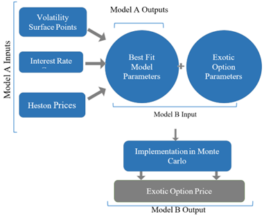
There are no obtainable market prices to be detected because the primary market utilized for exchanging the most exotic options is the over-the-counter market. Therefore, compared to their vanilla counterparts, exotic option prices are more sensitive to the model specification. This paper tries to rationalize the pricing methods and minimize the ambiguity caused by complex mathematical models by integrating the required inputs with market factors that reflect market sentiments towards the product risk profile at a point in time. The proposed methodology consists of a two-step model: As displayed in Figure 1, Model A defined by step 1 to 3 below that will become an input model to Model B described in steps 4 and 5:
Figure 1. Illustrated model scheme
1. Defined f the Heston function as fHeston with arguments of s, St, K, r, T, sigma, kappa, theta, vega and rho that illustrated our inputs and the model parameters {σ, k, θ, v, ρ} respectively;
2. Computed the integral of fHeston function by selecting a large limit that allows our integral to converge, resulting our Heston Pricing Model;
3. Started with the calibration process:
a. Assembled datasets containing option inputs and presented values using a web scrapping scheme from yahoo finance.
b. Constructed the volatility surface using the imported data (days to maturity, strike price, vanilla call option prices).
c. Obtained the last available risk-free rates using treasury rates from the CNBC website.
d. Applied the interpolation methodology to acquire our risk-free curve.
e. Constructed a vector function in order to compute the prices of all options consistent with the ordinary points on the volatility surface using the Heston Pricing Model.
f. Heston’s parameters fit the points of the volatility surface using a reiterative process that minimizes the square error between all estimated prices utilizing the market prices and our model.
4. For every set of parameters obtained from Model A, we calculated the moving average of stock price, known as the drift value, that will be an input for Model B.
5. Using the obtained drift, the exotic option prices were calculated via Monte Carlo replication with 100,000 iterations.
2.2 Sampling technique and sample size
As the prices of exotic options could not be accessed, we utilized a dataset of vanilla option prices for S&P 500 index futures, covering the period from November 10, 2022, to December 17, 2027. This dataset was chosen for several reasons. First, it allows for meaningful comparison with previous literature studies focused on index options [3, 23, 24]. Second, index options provide a more comprehensive representation of the overall economy compared to individual stocks traded actively in the market.
For this stage of the study, we selected option Greeks as a sample of vanilla option prices for the S&P 500. Using this data, we created a volatility surface by plotting strike prices, option prices, and days to maturity. We considered approximately 90% of the available days to maturity values for the volatility surface, and for each expiration date, we used 15 sample values for the option strike price, including at-the-money, in-the-money, and out-of-the-money values. The sample size can be adjusted based on the platform's capacity to handle data processing, and in general, larger sample sizes yield better model performance and results. The sample consisted of 675 contract prices, varying based on the expiration date and strike price.
To determine risk-free rates, we imported treasury rates from cnbc.com and constructed a risk-free curve using interpolation. It's important to note that our model was calibrated using current market data, distinguishing it from Hull and Suo's model, which relies on a "true" model for generating exotic and vanilla option datasets. This approach allows for benchmarking between the realized prices and our model's results. The main factors influencing our model and its output are the calibration procedures for each stock evaluation and the input values for each exotic option characteristic.
2.3 Tools and techniques of data collection
An open-source dataset is absent because the historic vanilla options information and their numerous tenders are incredibly assorted. Accordingly, an automatic procedure was exploited to acquire option prices using a web scrapping approach from Yahoo Finance to execute our data collection in a dynamic behavior on each code run. This procedure maintains access to a database with the daily trading outcomes of all listed option contracts and their corresponding security prices without uploading any file containing those prices.
This data was supplemented with treasury yields obtained from the CNBC website, which will inform the risk-free rate for our model. The interpolation procedure was used to compute the risk-free rate curve and alter the technique that prior studies have frequently directed. Numerous models match the crop on the US Treasury instrument considering maturity much closer to each option's expiration time.
Additionally, because the trade data only includes the contract's inner bid and ask values, the mid-price (average of the two) was used as a label for the option's fair value. Prior investigations led by Anders et al. [25], Bennell and Sutcliffe [26] and Stark [27] advocate the convention of exclusion principles to eliminate “non-representative” instances symbolizing unanticipated or illiquid options’ situations [26-28]. These filters eliminate options that are too far in-the-money or out-of-the-money, have an expiration date longer than five years, or are traded at such low values that the discrete character of security prices comes into play. In this study, it was decided on a certain number of strikes close to the money to pass these limitations.
2.4 Empirical framework
This section will be reconnoitering and elucidating the separate phases implemented to assemble the outcomes via aggregating the financial, mathematical, and programming fields.
2.4.1 Building the Heston model
The Heston Pricing Formula for a call option:
$C=S_t \cdot P_1\left(S_T>K\right)-K e^{-r t} \cdot P_2\left(S_T>K\right)$
Where the extended form is:
$\begin{gathered}C=S_t \cdot\left[\frac{1}{2}+\frac{1}{\pi} \int_0^{\infty} \operatorname{Re}\left[\frac{e^{-i s \ln K} f_1(s, v, x)}{i s}\right] d s\right]-K e^{-r t} \cdot\left[\frac{1}{2}\right. \left.+\frac{1}{\pi} \int_0^{\infty} \operatorname{Re}\left[\frac{e^{-i s \ln K} f_2(s, v, x)}{i s}\right] d s\right]\end{gathered}$
The previous function contains two integrals and a Re that condenses the complete integral. This concludes that the results will be in the imaginary complex form, so we will only represent the price with the real number part. As known, i is used as a definition of the complex number of the square of negative values ($i=\sqrt{-1}$). Each integral result in a function fj, defined as:
$f_i(S, v, x)=\exp \left(C_i(\tau, s)+D_j(\tau, s) \cdot v+i . s . x\right)$
C and D are defined as:
$\begin{gathered}C_j(\tau, s)=r . i . s . \tau+\frac{a}{\sigma^2}\left[(B R S) \cdot \tau-2 \ln \left(\frac{1-g_j \cdot e^{d_j \cdot \tau}}{1-g_j}\right)\right] \\ D_j=\frac{B R S}{\sigma^2}\left(\frac{1-e^{d_j \cdot \tau}}{1-g_j \cdot e^{d_j \cdot \tau}}\right)\end{gathered}$
And assuming:
$\begin{gathered}x=\ln S_t \\ d_j=\sqrt{(\rho . \sigma . i . s)^2-\sigma^2 \cdot\left(2 \cdot u_j . i . s-s^2\right)} \\ g_j=\frac{b_j-\rho \cdot \sigma \cdot i . s+d_j}{b_j-\rho \cdot \sigma \cdot i . s-d_j}\end{gathered}$
where, u1=0.5, u2=0.5, and b1=k-ρ.σ, b2=k.
BRS element is defined by:
$B R S=b_j-\rho . \sigma . i . s+d_j$
Everything was combined into one integral and one function f rather than being divided into two integrals:
$\begin{aligned} C=\frac{1}{2}\left(S_t-K e^{-r(T-t)}\right) +\frac{1}{\pi} \int_0^{\infty} \operatorname{Re}\left[e^{r(T-t)} \frac{f(s-i)}{i s . K^{i s}}\right. \left.-K \frac{f(s)}{i s . K^{i s}}\right] d s\end{aligned}$
f defined with:
$\begin{aligned} f(x)=e^{i x r T} S_t^{i x} & \left(\frac{1-g \cdot e^{d \cdot \tau}}{1-g}\right)^{-\frac{2 k \theta}{\sigma^2}} \times \exp \left[\frac{\tau k \theta}{\sigma^2}(k-\sigma \rho \cdot i \cdot x-d)+\frac{v}{\sigma^2}(k\right. \left.-\sigma \rho \cdot i \cdot x-d) \frac{1-e^{d_j \cdot \tau}}{1-g_j \cdot e^{d_j \cdot \tau}}\right]\end{aligned}$
Assuming that:
$\mathrm{d}=\sqrt{(\rho \cdot \sigma \cdot \mathrm{i} \cdot \mathrm{x})^2-\sigma^2 \cdot\left(2 \cdot \mathrm{i} \cdot \mathrm{x}-\mathrm{x}^2\right)}, g=\frac{k-\rho \cdot \sigma \cdot i \cdot x+d}{k-\rho \cdot \sigma \cdot i \cdot x-d}$
fHeston is referred by f with inputs St, s, K, r, T, $\sigma, \kappa, \theta, v$, and ρ. i were deliberated as a global variable since complex numerical values were strictly used in our function. Each complex number was fundamentally an action on i in which the function is protracted, calculating d and g. Then, the large exponential f(x) is cracked down and fragmented into two segments of the exponential function rendering it less complex to distribute the product of both exponentials gaining the complete fHeston function.
Since it is not possible for something to constantly operate because our integral extends to infinity, selecting a significant bond that permits our integral to converge was a must. By convergence, the supplementary zones under the computed curvature are so finite that they are regarded as negligible. In this model, a hundred was nominated. However, this number can be changed to detect sensitivity and performance. To calculate the integral function, our area was divided into rectangles discovering the mid-point, which will be utilized to compute each rectangle’s area, followed by summating all the areas. Our model initialized P the final price values to 0. Then, the areas were fragmented into 1,000 rectangles setting the limit to 100. In the core, the width of each rectangle will be du=100/10000. Subsequently, the first part of the Eq. (1) was calculated before the integral.
Thereafter, two variables were defined which are s1 and s2 as stated in the formulation. Increments of s1 are obviously detected at each iteration of the loop. For instance, s1=du*(2*1+1)/2 leading to s1=du*1.5 when j=1. On the other hand, s1=du*(2*2+1)/2 leading to s1=du*2.5 when j=2. Both examples prove our midpoint rule cast-off for the integration. Another reason we did not start from 0 is due to the fact that close attainment to the null value may mean dividing a number by 0, which would indeed be problematic. At this stage, the rectangles’ widths are considered in which the height is basically the value extracted from the fHeston function when changing the x-value intercept. The summation of all results extracted from fHeston and divided by the denominator are deliberated as heights. In conclusion, the areas now can be computed and summed together.
2.4.2 The role of calibration
Calibration should be mandatorily performed to make a pertinent model to actual markets appropriate for fiscal evaluation alongside transaction and risk management. These parameters were utilized in the mechanisms of pricing complex and exotic options. Unfortunately, discovering a locked arrangement formulary for estimating exotic options was difficult due to the presence of very intricate categories of options. For the aim of finding the parameters of the Heston model, plain vanilla options were used. On the other hand, the attained factors from the marketplace to compute the monetary value of the exotic options were utilized via implementing the Monte Carlo simulation model.
Having options with different expiries and maturities was considered when conducting the calibration procedure. One set of parameters is possessed for the whole set of options. However, sensitivities cannot be accumulated if a model occurs for each point since it is fundamentally an assessment between apples and oranges. Commencing with a parameter array ($\sigma=0.1, \kappa=0.1, \theta=0.1, \rho=0.1, v=0.1$), the Heston prices were computed for all categories of options followed by calculating the squared error between the forecasted prices by the Heston model and the actual market prices. Afterward, a solver was utilized in order to lessen the error to the extent of becoming negligible, which can be implemented on Microsoft Excel ®. Finally, options will be financially evaluated via the optimal parameters and the Monte Carlo simulation approach.
The first step consists of obtaining option quotes which can be collected either by scraping the quotes online or directly from any accessible online source. The first option was chosen for our model in order to add dynamics to it as well. However, option quotes typically do not go out very long into the future since it would be very difficult to analyze the shape of the marketplaces in the next decade due to the maturities of bonds that can go to infinity, such as permanency bonds. Options constructed on static revenue products are disposed to go out very long into the impending timelapse contrasting from option quotes only in the case with bonds.
The S&P 500 index options were used to calibrate our Heston model. The calibration is probably directed with any particular stock partaking in adequate quoted options. To acquire the options’ prices, we introduced an “options” bundle from the “yahoo_fin” library. Furthermore, the Pandas library is used to organize the obtained data as tabulations. A blank " surface " list was formed, which includes all the quotes as an assorted array. A maturity date will be accessible fundamentally by each component list. Since we are focusing on mutual strikes, all lists are equivalent in length. The dateIndex encompassed the maturity dates. To compute the maturity dates relative to today in the unit of years, we will be consuming these maturity dates which are comprised in the dateIndex. Similarly, the option quotes were added to this surface. Finally, the volatility surface was defined by observing 15 different strike prices and forty-five different maturity times. These maturity/moneyness amalgamations combined offer 675 “standard” points on the volatility surface.
The same structure to detect the risk-free curvature was used as well. The treasury degrees extracted from the CNBC website were used via the scraping method to maintain the dynamics of our model in which the most current possible rates were extracted. Then, all rates were converted to floating alongside changing the time to maturity vector:
From: [ $1 \mathrm{M} \,\,\,3 \mathrm{M}\,\,\, 6\mathrm{M}\,\,\, 1 \mathrm{Y}\,\,\, 2 \mathrm{Y}\,\,\, 3 \mathrm{Y}\,\,\, 5 \mathrm{Y}\,\,\, 7 \mathrm{Y}\,\,\, 10 \mathrm{Y}\,\,\, 20 \mathrm{Y}\,\,\, 30 \mathrm{Y}$]
To: $\left[\frac{1}{12}, \frac{3}{12}, \frac{6}{12}, 1,2,3,5,7,10,20,30\right]$
Next, interpolation is applied in order to obtain the interest rate curve. However, this step is very vital as it aids in evaluating the rate corresponding to each maturity. Nelson Siegel Svensson's method was used to smear this interpolation. This method is deliberated as one of the most recognized practices for interpolating a curve.
The calibration process started by setting up the parameters which were used to determine the coherence of our Heston model. The surface is transformed into an array of quotes containing strike, maturity, and quotes associated with each horizontal row. DIFHest is also a simple function that distributes a vector of differences between the prices obtained from the market and gained from our model. Consequently, the errors were squared and summed on each iteration to cast what is called the summation of squared errors when we converge with our optimization algorithm. This is how the algorithm function can resume the process of minimizing the error until reaching an optimal solution. For the sake of optimizing the functions’ evaluations, few elements from the Numba library were also added since the computations will be fastened in the calibration process:
Error $=($MarketPrices - ModelPrices$) /$ MarketPrices
The inputs are: (Algorithm values in this order: [sigma, kappa, theta, vega, rho])
Initial values (Default value: [0.1, 0.1, 0.1, 0.1, 0.1])
Lower bounds for our values (Default value: [0.001, 0.001, 0.001, 0.001, -1.00])
Upper bounds for our values (Default value: [1.0, 1.0, 1.0, 1.0, 1.0])
Volatility surface
Risk-free curve
Stock price (St today)
This calibration is lengthy in the time constraint since the option surface comprises 675 points necessitating about 20 minutes. The number of options can be abridged or executed as an approximation. Then, the optimum factors will be procured, which should be equivalent to today’s stock prices.
2.4.3 Implementation in Python
For the purpose of executing the model in Python and defining the MCHeston function, the following will be conducted:
a. Defining the number of time steps desired annually in which dt could be daily, weekly, monthly or yearly. We designated just one timestep each month.
b. Determining the sum of recapitulations which we require for spawning ST 1000, 10000, or 100,0000 (iterations number).
c. Stating all the gaussians assisting in hurtling this code where we consume X amount of timesteps, which is our timesteps x maturity and alongside Y which is the sum of iterations.
d. Computing all vt simultaneously for each timestep. The NumPy bundle enables us to conduct vectorized computations rapidly.
e. Each vt [i,:] depends on the vt [i-1,:] that came before it, and the same is true for St [i,:]. The values vt are similarly determined first before being inserted into St.
f. Mean value of all ST will be deducted from K shadowed by reducing it at the rate of r on a ceaseless establishment in order to acquire the present value of our option.
g. The ampoules will be considered to grasp all the ideals of ST and $\alpha$. Additionally, the initial standards of ST will be today’s stock price in which $\alpha$ the primary worth should be the factor of $\sigma$.
h. All those steps lead us to calculate the drift value using the function MCHeston. This function takes as inputs:
$\left\lceil S_0, K, r, T\right.$, sigma, kappa, theta, vega, rho, iterations, time step $\rceil$ Drift $=\max ($MCHeston, 0)
i. The drift value will be implemented to the Monte Carlo simulation in our model, adding the needed parameters of the exotic options, the price will be calculated. Output prices are discussed in the next section.
In this study, we developed a model through deep analysis of theoretical frameworks, exploring its results and trustworthiness, and highlighting its dynamic nature. We collected market prices for a sample of 34 exotic options from a renowned market maker, providing a valuable benchmark for performance comparisons. The strength of our model lies in its recalibration at each trading moment, reflecting real-time market option pricing and allowing the model parameters to fluctuate over time. This provides a more accurate representation of the underlying asset return distribution compared to models with constant parameters. Tested on a variety of exotic options, our model demonstrated its versatility and superior performance, especially with the Asian and Up-and-Out options. These findings underline the potential of our dynamic model in enhancing the accuracy of exotic option pricing.
3.1 Results by option type
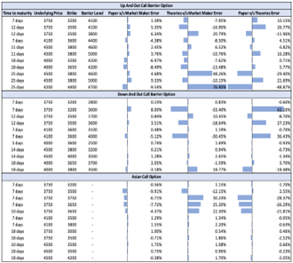
Three option types (Up-and-Out Barrier, Down-and-Out Barrier, and Asian), with different time-to-maturity values, underlying prices, strikes, and barrier levels) will be demonstrated. It is worth mentioning that the theoretical prices were conducted by yhe Black and Scholes model for the Asian options and by the trinomial model for the Barrier options.
3.1.1 Up-and-out barrier option
Table 1 shows three different calculated errors. First, the test is obtained by comparing our model's performance to the market, second by comparing the performance of the theoretical models to the market, and third by comparing our model prices to the theoretical prices.
According to Table 1, the average error of the difference between our prices and market prices is (0.36%). In contrast, the error between the prices obtained by the theoretical model, which is a trinomial model in this case, and the market prices is (7.01%). The variance is lower in our model compared to the theoretical one. The skewness and kurtosis calculated for our model are more indicative than the theoretical ones since they are closer to zero demonstrating the absence of fatty tails. Hence, our model is closer to a normal distribution, and the extreme errors are lower than those of the theoretical model. These results help validate our theory of establishing a model that takes theoretical models into account while including market sensitivity as an essential component to output the closest prices possible to the markets.
Table 1. Up-and-out parameters
|
Paper v/s Market Maker Error |
Theories v/s Market Maker Error |
Paper v/s Theories Error |
|
|
Mean |
0.36% |
7.01% |
-0.74% |
|
Standard Deviation |
0.07 |
0.30 |
0.22 |
|
Skewness |
-0.42 |
1.66 |
-1.06 |
|
Kurtosis |
-1.38 |
2.01 |
0.93 |
3.1.2 Down-and-out option
Similarly, we can conclude from Table 2 that our model is performing well compared to the market. With an average error of (0.82%), the error between the prices obtained by the theoretical model and the market prices is (-4.32%). When taking the standard deviation into account, we can deduce that our model is achieving lower error from the mean for each exotic price. Looking at skewness and kurtosis, we see that we have a lower skewness but a higher kurtosis. This indicates that the theoretical models are closer to a normal distribution. In addition, the error calculated between our model and the theories shows some variation. Nonetheless, we are still having decent results with a small average error, albeit to a lesser extent, when comparing our model (the Down-and-Out type) to other exotic option types which performed better.
Table 2. Down-and-out parameters
|
Paper v/s Market Maker Error |
Theories v/s Market Maker Error |
Paper v/s Theories Error |
|
|
Mean |
0.82% |
-4.32% |
8.91% |
|
Standard Deviation |
0.03 |
0.16 |
0.23 |
|
Skewness |
0.38 |
-0.81 |
1.40 |
|
Kurtosis |
1.92 |
-0.13 |
1.56 |
3.1.3 Asian options
Table 3 shows that our model is performing so much better than the theoretical models, as evidenced by a lower average and a very low standard deviation. The skewness and kurtosis values are negative but close to zero support our model and hypothesis. The two models in the Asian case seems to be performing well compared to the market.
Table 3. Asian parameters
|
Paper v/s Market Maker Error |
Theories v/s Market Maker Error |
Paper v/s Theories Error |
|
|
Mean |
-2.00% |
6.37% |
-6.67% |
|
Standard Deviation |
0.04 |
0.13 |
0.12 |
|
Skewness |
-0.97 |
0.94 |
-1.33 |
|
Kurtosis |
-0.56 |
0.06 |
-0.08 |
3.2 Discussions and interpretations
The exotic price of an option is a very critical subject, especially since the accuracy of the price is affected by several factors. Many researchers have tried to conduct accurate pricing using well-known reputable models for option pricing. Almost all the studies tried to apply different theoretical methods to address this problem, but the implementation of artificial intelligence escalated the pricing task to a new higher level. This paper has developed a model that considers the importance of the dynamic and sensitive behavior of the market by applying artificial intelligence.
Therefore, overall artificial intelligence has provided better results compared with other static models. This may be partly because artificial intelligence can capture the market's sensitivity better than other methods. Chen used a model of non-constant volatility by using the Heston model on a barrier option and another version by using Brownian motion without incorporating artificial intelligence [28]. The calculated error obtained by Chen [28]. was higher than ours. A higher sensitivity denotes a greater influence on how the predicted value varies in relation to the network's expected output. However, the model structure played a significant role in the accuracy of prices. Table 2 shows the error using all the available option prices to evaluate our model.
Figure 2. All exotic option prices
Table 4. All exotic option parameters
|
Paper v/s Market Maker Error |
Theories v/s Market Maker Error |
Paper v/s Theories Error |
|
|
Mean |
-0.33% |
3.12% |
0.29% |
|
Standard Deviation |
0.05 |
0.21 |
0.20 |
|
Skewness |
-0.32 |
1.49 |
0.51 |
|
Kurtosis |
-0.32 |
4.12 |
2.42 |
When comparing our model to the theoretical ones, the former has a lower average error (-0.33%), a lower standard deviation (0.05), and skewness and kurtosis that are closer to zero (Table 4). Hence, our model has a better performance than theoretical ones. This highlights the importance of a dynamic model, which takes into consideration the sensitivity of the market by building upon existing theoretical models.
To validate our model from a statistical view, we have used the two-sample Kolmogorov-Smirnov test, one of the most beneficial and versatile nonparametric techniques for evaluating two samples as it verifies if they are derived from the same distribution. This test does not report any confidence level since it does not compare any particular parameter (median, average). It is adequate for this study as it provides a dissimilarity parameter output of the best fitting sample (theoretical vs. our model) when compared to the original distribution (market prices in our case). The sample with the less dissimilarity value will be assumed to be the best fit for the original data. Dissimilarity will be calculated as follows: $D=\max _{1 \leq i \leq n}\left|\sum_1^i Y_i-\sum_1^i Z_i\right|$, where n represents the sample size.
Table 5. Dissimilarity values
|
Paper v/s Market |
Theories v/s Market |
Paper v/s Theories |
|
|
Dissimilarity Value |
103.66 |
388.44 |
368.27 |
Based on the dissimilarity value mentioned in Table 5, our model result is more similar to the market results when compared to those derived from the theoretical models. Among all the studies listed and analyzed in the literature review, the most similar approach to this study is the model calibration approach study by Babbar and McGhee [22] and Horvath et al. [9]. This study results are more effective due to the volatility surface plot. Furthermore, it tried to summarize all the advantages of the previous study in ours and waive their disadvantage by using a neural network. On the other hand, the study by Mezofi and Szabo [17] introduced machine learning and neural network to release the volatility of Black and Scholes of its static status, but failed to mention any output concerning the exotic option price. Therefore, it can be advantageous when compared to theoretical model by being closer to the market, but also still aligned with the theory. This is achieved by incorporating more realistic variables which instantly takes the market sentiment.
3.3 Limitations and future research
Despite our model's promising performance in exotic option pricing, we faced limitations including data unavailability and memory constraints of Google Colaboratory. We had restricted access to market prices for exotic options, limiting our sample size to 34, and our memory capacity limited the number of vanilla option prices and Monte Carlo iterations we could utilize. Our research hints at promising future directions including automation in parameter calibration, ensemble modeling, and expanding testing to put options and different exotic options. Alternatives like the Bates model could potentially enhance performance, and implementing a neural network model may further improve pricing accuracy. These future directions aim to overcome current limitations and bring us closer to a more accurate and comprehensive exotic option pricing model.
This study introduces an AI model that tackles real-world complexities in the pricing of exotic options, taking into account direct relationships with the volatility surface and option parameters. The model integrates data from 675 vanilla call option prices for the S&P 500, the risk-free rates curve, and a constructed volatility surface. Testing has demonstrated significant advancements towards market prices, as evidenced by reduced error variances, low skewness, near-zero kurtosis levels, and Kolmogorov-Smirnov analysis. Theoretical models have been expanded upon with our dynamic model that accounts for market sensitivity. While our model approximates the market more closely, it remains in alignment with theoretical models and can be adapted to other contract types and exotic options. It rapidly computes prices for three types of exotic options with minimal error, considering the same variables impacting standard option pricing. The implementation of multiple models enhances the pricing of exotic options.
4.1 Theoretical implications
Option pricing research frequently focuses on vanilla options, with a smaller number of studies addressing the complexities of exotic options. Existing studies typically employ constant-parameter models to evaluate out-of-sample pricing and hedging, whereas practitioners adjust models daily to correspond with market fluctuations. This disparity prompted the proposal for a new methodology that does not rely on historical exotic option data. Instead, collaboration with investment banks was initiated to align our model with real market prices, thus fostering practical application.
Previous research, such as Cao et al., valued exotic options based on volatility surfaces, yet neglected the significance of market prices [29]. In a similar vein, Kingma and Ba developed neural network models with a sole emphasis on model risk [30]. Conversely, our approach maintains the relevance of theoretical models while affording a fresh comparative perspective. By integrating the established Heston and Monte Carlo models, a dynamic, reliable model has been created. The accuracy of our findings is corroborated by minimal volatility and smaller spreads between over-the-counter prices and the outputs of our model, exceeding conventional mathematical models.
4.2 Practical implications
This study bridges the gap between market and theory prices, eschewing the use of static parameters and highlighting practical implications. Our model, capable of accurately predicting exotic prices, caters to academics, researchers, and market companies, including investors, banks, and market makers. It serves not only as a benchmark for option pricing, but also provides guidance in determining transaction costs and commissions. The model extends its usefulness to traders, aiding in the formulation of profitable portfolios by predicting exotic option prices. Thus, our research extends beyond academic confines, offering tangible applications, particularly within the financial industry.
[1] Liu, K., Wang, X. (2013). A pragmatical option pricing method combining Black-Scholes formula, time series analysis and artificial neural network. In 2013 Ninth International Conference on Computational Intelligence and Security, pp. 149-153. https://doi.org/10.1109/CIS.2013.38
[2] Merton, R.C. (1976). Option pricing when underlying stock returns are discontinuous. Journal of Financial Economics, 3(1-2): 125-144. https://doi.org/10.1016/0304-405X(76)90022-2
[3] Bates, D.S. (1991). The crash ofʼ87: Was it expected? The evidence from options markets. The Journal of Finance, 46(3): 1009-1044. https://doi.org/10.1111/j.1540-6261.1991.tb03775.x
[4] Hull, J., White, A. (1987). The pricing of options on assets with stochastic volatilities. The Journal of Finance, 42(2): 281-300. https://doi.org/10.1111/j.1540-6261.1987.tb02568.x
[5] Heston, S.L. (1993). A closed-form solution for options with stochastic volatility with applications to bond and currency options. The Review of Financial Studies, 6(2): 327-343. https://doi.org/10.1093/rfs/6.2.327
[6] Jaderberg, M., Mnih, V., Czarnecki, W.M., Schaul, T., Leibo, J.Z., Silver, D., Kavukcuoglu, K. (2016). Reinforcement learning with unsupervised auxiliary tasks. arXiv preprint arXiv:1611.05397. https://doi.org/10.48550/arXiv.1611.05397
[7] Chen, W., Shahabi, H., Shirzadi, A., Hong, H.Y., Akgun, A., Tian, Y.Y., Zhu, A.X., Li, S.J. (2019). Novel hybrid artificial intelligence approach of bivariate statistical-methods-based kernel logistic regression classifier for landslide susceptibility modeling. Bulletin of Engineering Geology and the Environment, 78: 4397-4419. https://doi.org/10.1007/s10064-018-1401-8
[8] McGhee, W. (2020). An artificial neural network representation of the SABR stochastic volatility model. Journal of Computational Finance, 25(2). https://doi.org/10.2139/ssrn.3288882
[9] Horvath, B., Muguruza, A., Tomas, M. (2021). Deep learning volatility: A deep neural network perspective on pricing and calibration in (rough) volatility models. Quantitative Finance, 21(1): 11-27. https://doi.org/10.1080/14697688.2020.1817974
[10] De Spiegeleer, J., Madan, D.B., Reyners, S., Schoutens, W. (2018). Machine learning for quantitative finance: fast derivative pricing, hedging and fitting. Quantitative Finance, 18(10): 1635-1643. https://doi.org/10.1080/14697688.2018.1495335
[11] Hutchinson, J.M., Lo, A.W., Poggio, T. (1994). A nonparametric approach to pricing and hedging derivative securities via learning networks. The Journal of Finance, 49(3): 851-889. https://doi.org/10.1111/j.1540-6261.1994.tb00081.x
[12] Kakkad, J., Makwana, S., Shah, R., Chachra, S. (2019). Real time predictive analysis of Indian stock market using machine learning and natural language processing. International Research Journal of Computer Science (IRJCS). https://doi.org/10.26562/irjcs.2019.apcs10088
[13] Dugas, C., Bengio, Y., Bélisle, F., Nadeau, C., Garcia, R. (2000). Incorporating second-order functional knowledge for better option pricing. Advances in Neural Information Processing Systems, 13. https://doi.org/10.5555/3008751.3008817
[14] Hahn, J.T. (2013). Option pricing using artificial neural networks: An Australian perspective. Doctoral dissertation, Bond University. https://doi.org/10.5555/3008751.3008817
[15] Audrino, F., Colangelo, D. (2008). Forecasting implied volatility surfaces. University of St. Gallen, Department of Economics, Discussion Paper, (2007-42). http://doi.org/10.2139/ssrn.1031859
[16] Fang, Z., George, K.M. (2017). Application of machine learning: An analysis of Asian options pricing using neural network. In 2017 IEEE 14th International Conference on e-Business Engineering (ICEBE), pp. 142-149. https://doi.org/10.1109/ICEBE.2017.30
[17] Mezofi, B., Szabo, K. (2018). Beyond black-Scholes: A new option for options pricing.
[18] Yao, J., Li, Y., Tan, C.L. (2000). Option price forecasting using neural networks. Omega, 28(4): 455-466. https://doi.org/10.1016/S0305-0483(99)00066-3
[19] Ferguson, R., Green, A. (2018). Deeply learning derivatives. arXiv preprint arXiv:1809.02233. https://doi.org/10.48550/arXiv.1809.02233
[20] Broström, A., Kristiansson, R. (2018). Exotic derivatives and deep learning. https://doi.org/10.48550/
[21] Ferguson, R., Green, A. (2018). Deeply learning derivatives. arXiv preprint arXiv:1809.02233. http://dx.doi.org/10.2139/ssrn.3244821
[22] Babbar, K., McGhee, W.A. (2019). A deep learning approach to exotic option pricing under LSVol. University of Oxford Working Paper. 2019..
[23] Liu, S., Oosterlee, C.W., Bohte, S.M. (2019). Pricing options and computing implied volatilities using neural networks. Risks, 7(1): 16. https://doi.org/10.48550/arXiv.1901.08943
[24] Liu, S., Borovykh, A., Grzelak, L.A., Oosterlee, C.W. (2019). A neural network-based framework for financial model calibration. Journal of Mathematics in Industry, 9: 1-28. https://doi.org/10.1186/s13362-019-0066-7
[25] Anders, U., Korn, O., Schmitt, C. (1998). Improving the pricing of options: A neural network approach. Journal of forecasting, 17(5-6): 369-388. https://doi.org/10.1002/(SICI)1099-131X(1998090)17:5/63.0.CO;2-S
[26] Bennell, J., Sutcliffe, C. (2004). Black–Scholes versus artificial neural networks in pricing FTSE 100 options. Intelligent Systems in Accounting, Finance & Management: International Journal, 12(4): 243-260. https://doi.org/10.2139/ssrn.544882
[27] Stark, L. (2017). Machine learning and options pricing: A comparison of Black-Scholes and a deep neural network in pricing and hedging DAX 30 index options. Corpus ID: 53688283.
[28] Chen, Z. (2013). Pricing and hedging exotic options in stochastic volatility models. Doctoral dissertation, London School of Economics and Political Science.
[29] Cao, J., Chen, J., Hull, J., Poulos, Z. (2022). Deep learning for exotic option valuation. The Journal of Financial Data Science, 41(1): 41-53. https://doi.org/10.3905/jfds.2021.1.083
[30] Kingma, D.P., Ba, J. (2014). Adam: A method for stochastic optimization. arXiv:1412.6980. https://doi.org/10.48550/arXiv.1412.6980