Alek Nur Fatman![]() | Tohari Ahmad*
| Tohari Ahmad*![]() | Ntivuguruzwa Jean De La Croix
| Ntivuguruzwa Jean De La Croix![]() | Md. Sagar Hossen
| Md. Sagar Hossen![]()
© 2023 IIETA. This article is published by IIETA and is licensed under the CC BY 4.0 license (http://creativecommons.org/licenses/by/4.0/).
OPEN ACCESS
Advancements in information and communication technology have facilitated diverse operational environments, spanning across financial to military sectors. However, these advancements carry an escalation in cybersecurity threats, potentially compromising user privacy and security. Among the various mechanisms introduced to mitigate these threats, data hiding methods stand out. These methods embed covert data within cover data, such as audio and video files, thereby providing an additional layer of security. In this study, we develop upon the existing data hiding techniques, enhancing their capacity to conceal varied sizes of covert data. Our proposed method leverages both right and bottom context pixels for a more nuanced data hiding approach. The effectiveness of this scheme is evaluated by quantifying the quality of the stego data, represented by the Peak Signal to Noise Ratio (PSNR) value. Our initial findings indicate that our method yields superior stego data quality, suggesting its potential to accommodate a larger volume of covert data while preserving the similarity between the cover and stego files. This study thus contributes to more robust and efficient data hiding techniques, bolstering cybersecurity measures in the face of increasing digital threats.
data hiding, cyber security, histogram shifting, steganography, Peak Signal to Noise Ratio (PSNR), information security, network infrastructure
The rapid advancement of information technology has precipitated the swift development of computer networks, largely facilitating data transfer between devices. This progress, ubiquitous in nature, is uncompromised by location or time, provided network availability. A plethora of applications, compatible with various devices like smartphones and laptops, have been designed to cater to user demands, bolstered by the supportive services offered by software and hardware companies.
However, this technological progress is not without its drawbacks. Security has consistently emerged as a significant concern, primarily due to the potential exploitation by third parties leveraging user unawareness. This could potentially lead to the public disclosure of user privacy. As such, mechanisms to safeguard covert data are paramount. Several methodologies have been introduced to address this issue, including the development of Intrusion Detection Systems [1, 2], message encryption [3, 4], and data embedding techniques [5, 6].
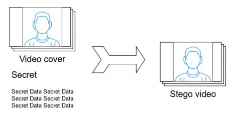
Data embedding involves the integration of covert data into a cover file, such as an image or audio file (illustrated in Figure 1). The challenge lies in ensuring the generated stego file bears resemblance to the cover file. This method, since its introduction, has encountered numerous challenges, including maintaining the quality of the stego file and determining the size of the covert data that the cover file can accommodate. While existing methods have shown improvements over their predecessors, there remains a persistent need for increased covert data size and improved stego file quality, contingent on the respective environment. A typical trade-off between the size of covert data and the quality of the stego file has been identified, necessitating user focus on one of these aspects.
Ni et al. [7] introduced the concept of histogram shifting, applicable to both images and video files, considering that videos are essentially a compilation of pixel-containing frames. The peak and zero points are defined, determining the direction of the shifting process. However, this process affects the quality of the stego file, as pixel values within specific ranges are affected. Moreover, excessive pixel shifting is likely to degrade the stego file quality.
Subsequent research developed a prediction error (PE) between two sequential frames [8]. The PE value is derived from the difference between corresponding pixels in the frames, generating a histogram where the embedding process is to be conducted. Similar to prior research, the shifting direction is determined to provide the embedding space.
In contrast, Qu and Kim [9] adopted a different approach, Pixel based Pixel Value Ordering (PPVO), wherein an image is divided into context pixels of predetermined sizes (such as 2×2 or 4×4). The minimum and maximum values of each context pixel are obtained to predict a value for embedding. The considered pixel in each image is compared to the minimum value for this prediction. The value is equal to either the minimum or the maximum, depending on the result of this comparison.
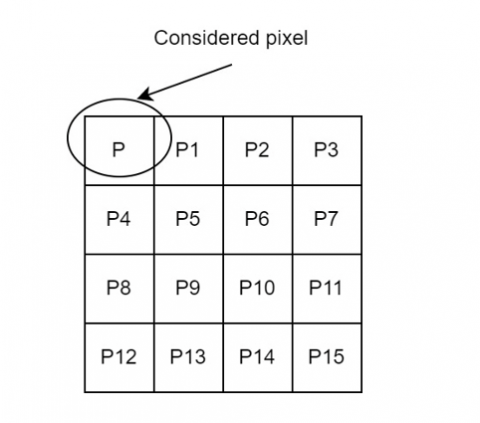
Drawing inspiration from Qu and Kim's research [9], we designed a method [10] that considers pixels to the right and bottom of the context (illustrated in Figure 2). The average of these values specifies the embedding process. This approach was found to enhance the performance of both Ni et al.'s and Qu and Kim's methods [7, 9], although it still slightly lags behind that of PE [8]. Various other data-hiding approaches can be found in studies [11-14], with specific purposes like Arabic text [15] and deep learning [16] also implemented. Techniques to break these data-hiding methods have been introduced [17, 18], perpetuating the competition between steganography (data hiding) and steganalysis [19].
In this study, we propose a video-based data-hiding method, improving upon previous methods by utilizing frames in the video file as the basis for embedding. A histogram is generated and the shifting direction is determined based on set criteria. Acknowledging the strengths and limitations of previous research, the proposed method aims to enhance the capacity to hide covert data. We continue to address two primary factors: the size of covert data and the quality of the stego file, as detailed in the following section.
This paper is structured as follows: Section 2 details the methodology of the proposed approach. Section 3 presents the experimental results, analysis, and discussion, including a comparison with other research. The conclusion is provided in Section 4.
Figure 1. General process of data hiding
Figure 2. Illustration of a context pixel
As previously described, this proposed method is developed by improving our proposed method [10], which extended [7, 8]. In the study [10], we take the average value of the bottom and right pixels. It is to enhance the HS method [7], which is done according to the direction of the pixel with the lowest frequency. In the NS method [8], the shift is made in the direction of prediction errors based on the most significant value.
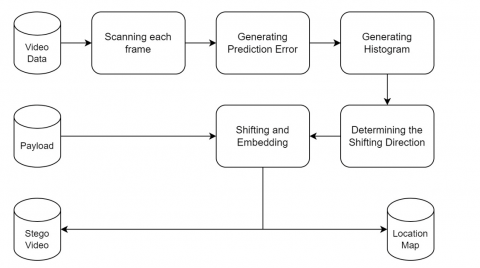
Differently, in this research, we arrange it based on the direction of pixels or prediction error with either the smallest frequency, the largest value, or the smallest value. The remaining payload, pixels or prediction errors that may be shifted and also the peak point value in the frame or prediction errors are taken to consider the shift direction. The illustration of this proposed process is given in Figure 3.
At the embedding stage, the video sample is processed to get all pixel values of each frame. The prediction error is searched for every two frames that are close to each other by reducing the pixel of a frame by the corresponding pixel in its subsequent frame (see Figure 4). Then, a histogram is created for each frame beside the first frame and each prediction error, where the shifting is performed. From each histogram, we determine four peak points and six zero points by considering the following factors:
Next, some values are specified based on those definitions, as in Eqs. (1)-(8).
$p_5=\max \left(p_1, p_3\right)$ (1)
$p_6=\min \left(p_1, p_2\right)$ (2)
$p_7=\max \left(p_2, p_4\right)$ (3)
$p_8=\min \left(p_2, p_4\right)$ (4)
$z_7=\left\{\begin{array}{l}z_1, \text { if } z_1>p_5 \\ z_3, \text { otherwise }\end{array}\right.$ (5)
$z_8=\left\{\begin{array}{l}z_1, \text { if } z_1<p_6 \\ z_2, \text { otherwise }\end{array}\right.$ (6)
$z_9=\left\{\begin{array}{l}z_4, \text { if } z_4>p_7 \\ z_6, \text { otherwise }\end{array}\right.$ (7)
$z_{10}=\left\{\begin{array}{c}z_4, \text { if } z_4<p_8 \\ z_5, \text { otherwise }\end{array}\right.$ (8)
It needs to get the value of the ith payload to be inserted (ϵi) by finding the lowest value of the ith peak point frequency (fpi) and the remaining payload (r) based on Eq. (9).
$\epsilon_i=\left\{\begin{array}{c}\min \left(f p_i+f p_{i-2}, r\right), \text { if } i=3 \text { or } i=4 \\ \min \left(f p_i, r\right), \text { otherwise }\end{array}\right.$ (9)
The moving direction in the embedding is determined based on the highest value obtained from Eqs. (10)-(17). The kth histogram value (hk) is determined by ϵ and the number of pixels si.j) having a value between the ith peak point (pi) and the jth zero point (zj).
$h_1=\frac{\epsilon_1}{s_{1.1}}$ (10)
$h_2=\frac{\epsilon_1}{s_{1.2}}$ (11)
$h_3=\frac{\epsilon_1}{s_{1.3}}$ (12)
$h_4=\frac{\epsilon_2}{s_{2.4}}$ (13)
$h_5=\frac{\epsilon_2}{s_{2.5}}$ (14)
$h_6=\frac{\epsilon_2}{s_{2.6}}$ (15)
$h_7=\frac{\epsilon_3}{s_{5.7}+s_{6.8}}$ (16)
$h_8=\frac{\epsilon_4}{s_{7.9}+s_{8.10}}$ (17)
Some highest h are selected, which are peak and zero points. If the selected h is either from h1, h2, h3, or h7, the shifting is performed in the frame; otherwise, in the prediction error. Here, all numbers between the peak and zero points are shifted toward zero points. In case the value of selected h is either h7 or h8, we select the highest peak point to be the top peak point, and the other is to be the bottom peak point. Next, all numbers higher than the top peak point are shifted to the right, and those less than the bottom peak point are to the left. According to the value of the payload bit, the peak point is shifted to the zero point; for either Eq. (16) or Eq. (17), the top peak point is shifted to the right, and the bottom peak point to the left.
For this experiment, fifteen videos taken from [20] are used for evaluation, whose examples are provided in Figure 5. Each video has 600 frames, sizing 176×144. They are to be embedded using various payload sizes: 1, 10, 20, 30, 40, 50, 60, 70, 80, 90, and 100 kb. Furthermore, we compare the performance of this proposed method to that of other existing methods of Ahmad et al. [10], Ni et al. [7], Yeh et al. [8], and Qu and Kim [9]. Similar to other research, PSNR is used to evaluate the quality of the stego video.
The experimental results of the proposed method are provided in Table 1, while others are in Tables 2, 3, 4, and 5, which are HS [7], NS [8], PPVO [9] with 3 context pixels, and PPVO [9] with 5 context pixels, respectively. We find that the average of the obtained PSNR is 71.597 dB; the highest value, 91.82 dB, is obtained using Foreman after being embedded using 1 kb payload and the lowest PSNR value, 62.84 dB, is from Coastguard containing 100 kb. It is shown that along with the increase in the payload size, the PSNR value decreases. Some video covers have lower PSNR values even though they are embedded by less payload size, such as Akiyo with 10 kb and Silent with 1kb. It happens because when choosing the direction of shifting, the value of the number of shifted pixels is proportional to the number of peak points; at the same time, the PSNR calculation is not comparable. In this method, the most influencing factor on the quality of the stego video is the number of shifted pixels, which have values between peak and zero points. The closer the peak point to the zero point, the better the quality of the stego video.
The experiment shows that HS [7] has lower PSNR. It is because it shifts all values between the peak and zero points, whose number is almost the same as the payload size to embed. It is worth noting that the more payloads being embedded, the more pixels are shifted because their value is between the peak and zero points. On the other hand, the PSNR of NS [8] is closer to that of the proposed method. Different from HS, NS only shifts the prediction error whose value is higher than the peak point in the respective prediction error. Because the shifted prediction error values are higher than the peak point, the quality of their stego video is less than that of the proposed method.
PPVO [9] using both 3 and 15 context pixels has higher PSNR values than HS [7] but still less than both NS [8] and the proposed method. We find that the proposed method has the highest average PSNR increase than the PPVO method, specifically in Silent video. Here, there is an increase of 12% from PPVO 3 context pixels, and 10% from PPVO 15 context pixels. The proposed method is also better than our previous research [10], considering that this study is developed by refining some weaknesses in that research.
Figure 5. Videos taken for the cover [20]
Table 1. PSNR values of the proposed method
|
Video |
PSNR Value (dB) from Various Payload Sizes (kb) |
||||||||||
|
1kb |
10kb |
20kb |
30kb |
40kb |
50kb |
60kb |
70kb |
80kb |
90kb |
100kb |
|
|
Akiyo |
78.21 |
70.29 |
78.07 |
76.60 |
75.40 |
74.50 |
73.73 |
73.10 |
68.95 |
71.93 |
71.50 |
|
Bowing |
83.56 |
79.76 |
77.63 |
76.23 |
75.11 |
74.26 |
73.53 |
72.93 |
72.24 |
71.74 |
71.33 |
|
Carphone |
78.02 |
74.53 |
73.78 |
70.95 |
70.59 |
69.05 |
68.81 |
67.84 |
67.75 |
67.56 |
66.94 |
|
Claire |
77.35 |
76.10 |
75.05 |
74.22 |
73.50 |
72.01 |
71.60 |
71.27 |
70.97 |
70.66 |
69.89 |
|
Coastguard |
75.40 |
73.22 |
70.18 |
68.35 |
66.41 |
65.60 |
64.52 |
64.33 |
63.71 |
63.22 |
62.84 |
|
Container |
80.75 |
78.57 |
76.88 |
75.68 |
74.68 |
73.91 |
73.23 |
71.74 |
71.36 |
70.96 |
70.61 |
|
Deadline |
78.69 |
73.75 |
73.11 |
68.78 |
70.38 |
70.09 |
67.72 |
68.66 |
68.47 |
68.25 |
66.19 |
|
Foreman |
91.82 |
81.66 |
72.52 |
69.99 |
69.70 |
68.18 |
66.99 |
66.85 |
66.72 |
65.78 |
65.13 |
|
Galleon |
74.17 |
74.04 |
73.37 |
71.17 |
70.80 |
70.47 |
70.15 |
69.13 |
68.92 |
68.68 |
67.05 |
|
Grandma |
79.34 |
77.62 |
76.31 |
75.34 |
74.51 |
73.80 |
72.63 |
72.14 |
71.71 |
71.27 |
70.90 |
|
Mother_daughter |
75.94 |
76.97 |
75.75 |
74.82 |
74.00 |
73.35 |
68.95 |
71.67 |
71.29 |
70.89 |
70.56 |
|
Pamphlet |
75.79 |
74.98 |
74.14 |
73.46 |
71.84 |
71.42 |
71.02 |
70.67 |
70.37 |
70.03 |
69.37 |
|
Paris |
77.07 |
73.33 |
69.61 |
70.38 |
70.06 |
68.63 |
68.41 |
68.24 |
67.31 |
67.14 |
67.01 |
|
Sign_irene |
77.38 |
76.12 |
75.07 |
74.24 |
73.50 |
71.47 |
71.07 |
70.72 |
70.40 |
70.13 |
69.12 |
|
Silent |
72.50 |
79.50 |
77.48 |
76.12 |
75.03 |
74.20 |
73.48 |
69.71 |
71.89 |
71.43 |
71.05 |
Table 2. PSNR values of the histogram shifting [7]
|
Video |
PSNR Value (dB) from Various Payload Sizes (kb) |
||||||||||
|
1kb |
10kb |
20kb |
30kb |
40kb |
50kb |
60kb |
70kb |
80kb |
90kb |
100kb |
|
|
Akiyo |
70.87 |
63.06 |
60.05 |
58.54 |
57.22 |
56.22 |
55.53 |
54.83 |
54.32 |
53.87 |
53.38 |
|
Bowing |
70.02 |
63.95 |
60.94 |
59.18 |
57.93 |
57.18 |
56.35 |
56.15 |
56.12 |
55.77 |
55.38 |
|
Carphone |
80.61 |
62.04 |
58.40 |
56.50 |
55.19 |
54.06 |
53.26 |
52.83 |
52.28 |
51.74 |
51.27 |
|
Claire |
70.48 |
67.33 |
65.53 |
64.26 |
63.28 |
61.85 |
61.26 |
60.74 |
60.28 |
59.86 |
59.15 |
|
Coastguard |
74.77 |
66.67 |
63.64 |
62.16 |
60.95 |
59.89 |
59.17 |
58.44 |
57.88 |
57.45 |
57.08 |
|
Container |
70.05 |
62.25 |
59.62 |
57.99 |
56.61 |
55.71 |
54.71 |
54.12 |
53.50 |
52.95 |
52.54 |
|
Deadline |
78.75 |
63.52 |
60.27 |
58.36 |
57.28 |
56.28 |
55.43 |
54.85 |
54.22 |
53.77 |
53.26 |
|
Foreman |
69.99 |
61.52 |
58.43 |
56.75 |
55.49 |
54.66 |
53.85 |
53.07 |
52.49 |
51.97 |
51.47 |
|
Galleon |
74.33 |
65.94 |
62.57 |
60.42 |
59.17 |
58.04 |
57.14 |
56.52 |
55.89 |
55.33 |
54.92 |
|
Grandma |
70.14 |
65.30 |
63.06 |
61.59 |
60.50 |
59.62 |
58.90 |
58.27 |
57.73 |
57.24 |
56.61 |
|
Mother_daughter |
75.94 |
68.09 |
65.25 |
63.68 |
62.72 |
61.78 |
60.86 |
60.19 |
59.63 |
59.22 |
58.76 |
|
Pamphlet |
69.96 |
62.17 |
60.36 |
58.46 |
57.14 |
56.14 |
55.47 |
54.76 |
54.26 |
53.71 |
53.22 |
|
Paris |
77.12 |
67.98 |
65.05 |
63.48 |
62.23 |
61.40 |
60.66 |
60.06 |
59.55 |
57.98 |
56.02 |
|
Sign_irene |
70.04 |
63.97 |
61.53 |
59.57 |
58.22 |
57.42 |
56.55 |
56.00 |
55.35 |
54.92 |
54.41 |
|
Silent |
72.50 |
61.48 |
57.84 |
55.93 |
54.76 |
53.71 |
52.91 |
52.23 |
51.68 |
51.30 |
50.85 |
Table 3. PSNR values of the neighboring similarity [8]
|
Video |
PSNR Value (dB) from Various Payload Sizes (kb) |
||||||||||
|
1kb |
10kb |
20kb |
30kb |
40kb |
50kb |
60kb |
70kb |
80kb |
90kb |
100kb |
|
|
Akiyo |
82.40 |
79.28 |
77.38 |
76.10 |
75.02 |
74.19 |
73.46 |
72.87 |
72.08 |
71.61 |
71.23 |
|
Bowing |
80.79 |
78.39 |
76.74 |
75.57 |
74.59 |
73.83 |
73.16 |
72.61 |
71.10 |
70.71 |
70.38 |
|
Carphone |
71.40 |
71.04 |
70.69 |
67.78 |
67.60 |
66.19 |
64.86 |
64.77 |
63.86 |
63.78 |
63.04 |
|
Claire |
74.35 |
73.68 |
73.05 |
72.51 |
72.01 |
70.05 |
69.75 |
69.49 |
69.26 |
69.00 |
68.78 |
|
Coastguard |
71.57 |
71.20 |
68.07 |
66.30 |
65.07 |
64.98 |
64.03 |
63.24 |
62.59 |
62.54 |
61.94 |
|
Container |
77.71 |
76.49 |
75.37 |
74.49 |
73.71 |
73.08 |
72.51 |
70.35 |
70.08 |
69.77 |
69.51 |
|
Deadline |
71.34 |
71.00 |
70.65 |
68.42 |
68.21 |
68.02 |
66.74 |
66.61 |
66.48 |
66.34 |
66.22 |
|
Foreman |
71.78 |
71.40 |
71.02 |
67.93 |
67.75 |
66.24 |
66.12 |
66.00 |
64.70 |
64.61 |
63.63 |
|
Galleon |
71.52 |
71.20 |
70.84 |
68.51 |
68.31 |
68.12 |
67.93 |
66.39 |
66.27 |
65.13 |
65.05 |
|
Grandma |
75.68 |
74.79 |
74.00 |
73.33 |
72.72 |
72.21 |
70.95 |
70.61 |
70.30 |
69.98 |
69.70 |
|
Mother_daughter |
75.58 |
74.70 |
73.92 |
73.27 |
72.67 |
72.16 |
70.41 |
70.10 |
69.83 |
69.54 |
69.28 |
|
Pamphlet |
72.74 |
72.26 |
71.80 |
71.39 |
69.91 |
69.64 |
69.37 |
69.13 |
68.91 |
68.67 |
68.12 |
|
Paris |
72.34 |
71.90 |
68.66 |
68.45 |
68.25 |
66.72 |
66.58 |
66.45 |
65.36 |
65.26 |
65.16 |
|
Sign_irene |
74.26 |
73.60 |
72.98 |
72.44 |
71.94 |
69.52 |
69.26 |
69.03 |
68.81 |
68.58 |
67.23 |
|
Silent |
80.11 |
78.05 |
76.51 |
75.38 |
74.45 |
73.71 |
73.05 |
71.47 |
71.12 |
70.73 |
70.40 |
Figure 6. Average PSNR values from various payload sizes
The average of the PSNR values taken by embedding various videos is provided in Figure 6. In this graph, the respective payload size is embedded in all covers. Overall, it is shown that the proposed method has the best results, followed by the NS [8]. On the other hand, HS [7] has the lowest results, and the PPVO [9] is between them. It can be inferred that the proposed method, in general, can work on both various covers and payload sizes. Therefore, it is more applicable to use than the others.
Nevertheless, it is worth noting that in specific cases, the others may be better than the proposed method. For example, NS [8] is more suitable for embedding 1 kb data to either Akiyo or Silent. It is predicted that those videos have different characteristics from others.
Table 4. PSNR values of the PPVO [9] with 3 context pixel
|
Video |
PSNR Value (dB) from Various Payload Sizes (kb) |
||||||||||
|
1kb |
10kb |
20kb |
30kb |
40kb |
50kb |
60kb |
70kb |
80kb |
90kb |
100kb |
|
|
Akiyo |
73.54 |
73.05 |
72.55 |
69.76 |
69.52 |
69.28 |
67.74 |
67.60 |
67.45 |
66.37 |
66.27 |
|
Bowing |
73.81 |
73.40 |
72.80 |
72.29 |
69.79 |
69.52 |
69.27 |
69.03 |
67.68 |
67.51 |
67.35 |
|
Carphone |
73.31 |
72.77 |
72.26 |
69.53 |
69.26 |
67.69 |
67.52 |
66.42 |
66.30 |
65.44 |
65.34 |
|
Claire |
74.37 |
73.82 |
73.35 |
72.93 |
72.64 |
70.23 |
70.01 |
69.81 |
69.66 |
69.51 |
68.14 |
|
Coastguard |
71.10 |
67.93 |
64.91 |
63.14 |
61.89 |
61.35 |
60.48 |
59.75 |
59.13 |
58.59 |
58.33 |
|
Container |
72.67 |
72.31 |
71.84 |
69.07 |
68.84 |
67.23 |
67.08 |
65.94 |
65.85 |
64.95 |
64.88 |
|
Deadline |
72.83 |
72.35 |
69.33 |
69.10 |
67.39 |
67.24 |
66.06 |
65.14 |
65.06 |
64.30 |
64.23 |
|
Foreman |
72.69 |
72.24 |
69.23 |
69.01 |
67.29 |
67.15 |
65.96 |
65.86 |
64.95 |
64.85 |
64.11 |
|
Galleon |
72.23 |
71.93 |
68.92 |
67.15 |
67.04 |
65.82 |
64.86 |
64.08 |
64.03 |
63.37 |
62.80 |
|
Grandma |
73.21 |
72.80 |
72.46 |
69.61 |
69.40 |
69.23 |
67.64 |
67.51 |
67.42 |
66.30 |
66.20 |
|
Mother_daughter |
73.49 |
72.98 |
72.48 |
69.72 |
69.47 |
69.24 |
67.72 |
67.57 |
67.42 |
66.35 |
66.24 |
|
Pamphlet |
72.23 |
71.88 |
68.85 |
68.64 |
66.93 |
66.79 |
65.61 |
65.50 |
64.60 |
63.84 |
63.77 |
|
Paris |
72.13 |
71.72 |
68.69 |
66.93 |
65.67 |
64.70 |
63.90 |
63.23 |
62.65 |
62.13 |
61.29 |
|
Sign_irene |
73.26 |
72.73 |
72.22 |
69.57 |
69.31 |
69.07 |
67.57 |
67.42 |
67.30 |
66.22 |
66.10 |
|
Silent |
72.08 |
71.68 |
68.67 |
66.92 |
65.66 |
64.69 |
63.90 |
63.83 |
63.18 |
62.61 |
62.10 |
Table 5. PSNR values of the PPVO [9] with 5 context pixel
|
Video |
PSNR Value (dB) from Various Payload Sizes (kb) |
||||||||||
|
1kb |
10kb |
20kb |
30kb |
40kb |
50kb |
60kb |
70kb |
80kb |
90kb |
100kb |
|
|
Akiyo |
74.97 |
74.35 |
73.68 |
70.97 |
70.65 |
69.08 |
68.89 |
67.77 |
67.65 |
66.76 |
66.66 |
|
Bowing |
75.47 |
74.89 |
74.07 |
73.39 |
71.05 |
70.70 |
70.37 |
68.99 |
68.83 |
68.59 |
68.39 |
|
Carphone |
74.50 |
73.82 |
70.83 |
70.50 |
68.83 |
67.64 |
67.47 |
66.57 |
66.45 |
65.71 |
65.61 |
|
Claire |
74.83 |
74.24 |
73.74 |
73.32 |
73.06 |
70.64 |
70.41 |
70.21 |
70.11 |
68.71 |
68.57 |
|
Coastguard |
74.53 |
69.47 |
67.21 |
65.19 |
64.19 |
63.07 |
62.43 |
61.65 |
61.18 |
60.58 |
60.21 |
|
Container |
74.72 |
74.16 |
71.11 |
70.84 |
69.14 |
68.96 |
67.80 |
67.67 |
66.80 |
66.67 |
65.95 |
|
Deadline |
75.30 |
74.49 |
71.52 |
69.77 |
68.51 |
67.55 |
67.39 |
66.63 |
65.99 |
65.42 |
64.92 |
|
Foreman |
75.25 |
74.49 |
71.45 |
69.65 |
68.37 |
68.20 |
67.24 |
66.45 |
65.80 |
65.68 |
65.12 |
|
Galleon |
74.45 |
74.04 |
71.07 |
69.33 |
68.07 |
67.10 |
67.02 |
66.24 |
65.60 |
65.02 |
64.52 |
|
Grandma |
75.31 |
74.71 |
74.24 |
71.44 |
71.18 |
70.95 |
69.41 |
69.27 |
68.17 |
68.04 |
67.94 |
|
Mother_daughter |
75.46 |
74.68 |
73.98 |
71.35 |
70.98 |
69.46 |
69.23 |
69.02 |
68.00 |
67.81 |
67.01 |
|
Pamphlet |
74.29 |
73.76 |
70.78 |
70.46 |
68.79 |
67.60 |
67.44 |
66.54 |
65.80 |
65.13 |
65.07 |
|
Paris |
74.92 |
71.65 |
69.83 |
67.68 |
66.25 |
65.64 |
64.69 |
63.91 |
63.55 |
62.93 |
62.63 |
|
Sign_irene |
74.67 |
73.96 |
73.41 |
70.76 |
70.41 |
68.91 |
68.69 |
67.64 |
67.47 |
67.36 |
66.50 |
|
Silent |
74.44 |
71.14 |
69.27 |
67.96 |
66.95 |
66.13 |
65.45 |
64.42 |
63.96 |
63.52 |
63.13 |
This study has enhanced the performance of existing data hiding methodologies. Drawing parallels to prior research, certain pixels were grouped into blocks. However, diverging from previous methods, specific directions for histogram shifting were defined. Experimental results have demonstrated that this proposed method generally augments the capacity for concealing covert data.
Future iterations of this method could potentially further improve stego quality or increase payload size. Such enhancements might be achieved through the identification of more suitable steps for determining the direction of histogram shifting. Additionally, a comprehensive analysis of the characteristics of the covers could elucidate which algorithms are best suited for specific covers. These covers could be categorized based on defined parameters, providing tailored solutions.
While the proposed method may necessitate complex calculations, potentially decelerating execution, it should be noted that this could pose a problem where time is a primary factor. Therefore, further refinement is still warranted to mitigate this issue.
The authors gratefully acknowledge financial support from the Institut Teknologi Sepuluh Nopember for this work, under project scheme of the Publication Writing and IPR Incentive Program (PPHKI) 2023.
[1] Pamungkas, I.G.A.K., Ahmad, T., Ijtihadie, R.M. (2022). Analysis of autoencoder compression performance in intrusion detection system. International Journal of Safety and Security Engineering, 12(3): 395-401. https://doi.org/10.18280/ijsse.120314
[2] Venkatraman, D., Narayanan, R. (2022). Integrated framework for intrusion detection through adversarial sampling and enhanced deep correlated hierarchical network. Revue d’Intelligence Artificielle, 36(4): 597-605. https://doi.org/10.18280/ria.360412
[3] Zou, C., Wang, X., Zhou, C., Xu, S., Huang, C. (2022). A novel image encryption algorithm based on DNA strand exchange and diffusion. Applied Mathematics and Computation, 430: 127291. https://doi.org.10.1016/j.amc.2022.127291
[4] Munir, N., Khan, M., Hussain, I., Alanazi, A.S. (2022). Cryptanalysis of encryption scheme based on compound coupled logistic map and anti-codifying technique for secure data transmission. Optik, 267: 169628. https://doi.org/10.1016/j.ijleo.2022.169628
[5] Hassan, F.S., Gutub, A. (2022). Novel embedding secrecy within images utilizing an improved interpolation-based reversible data hiding scheme. Journal of King Saud University - Computer and Information Sciences, 34(5): 2017-2030. https://doi.org/10.1016/j.jksuci.2020.07.008
[6] Benkhaddra, I., Kumar, A., Bensalem, Z.E.A., Hang, L. (2023). Secure transmission of secret data using optimization based embedding techniques in Blockchain. Expert Systems with Applications, 211: 118469. https://doi.org/10.1016/j.eswa.2022.118469
[7] Ni, Z., Shi, Y.Q., Ansari, N., Su, W. (2006). Reversible data hiding. IEEE Transactions on Circuits and Systems for Video Technology, 16(3): 354-362. https://doi.org/10.1109/tcsvt.2006.869964
[8] Yeh, H., Gue, S., Tsai, P., Shih, W. (2014). Reversible video data hiding using neighbouring similarity. IET Signal Processing, 8(6): 579-587. https://doi.org/10.1049/iet-spr.2012.0233
[9] Qu, X., Kim, H.J. (2015). Pixel-based pixel value ordering predictor for high-fidelity reversible data hiding. Signal Processing, 111: 249-260. https://doi.org/10.1016/j.sigpro.2015.01.002
[10] Ahmad, T., Fatman, A.N., Basori, A.H. (2021). Modified pixel value ordering-based predictor for reversible data hiding on video. In 2021 9th International Conference on Information and Communication Technology (ICoICT), Yogyakarta, Indonesia. https://doi.org/10.1109/ICoICT52021.2021.9527504
[11] Puteaux, P., Ong, S.Y., Wong, K.S., Puech, W. (2021). A survey of reversible data hiding in encrypted images – The first 12 years. Journal of Visual Communication and Image Representation, 77: 103085. https://doi.org/10.1016/j.jvcir.2021.103085
[12] AlSabhany, A.A., Ali, A.H., Ridzuan, F., Azni, A.H., Mokhtar, M.R. (2020). Digital audio steganography: Systematic review, classification, and analysis of the current state of the art. Computer Science Review, 38: 100316. https://doi.org/10.1016/j.cosrev.2020.100316
[13] Hussain, M., Wahab, A.W.A., bin Idris, Y.I., Ho, A.T.S., Jung, K.H. (2018). Image steganography in spatial domain: A survey. Signal Processing: Image Communication, 65: 46-66. https://doi.org/10.1016/j.image.2018.03.012
[14] Mandal, P.C., Mukherjee, I., Paul, G., Chatterji, B.N. (2022). Digital image steganography: A literature survey. Information Sciences, 609: 1451-1488. https://doi.org/10.1016/j.ins.2022.07.120
[15] Roslan, N.A., Udzir, N.I., Mahmod, R., Gutub, A. (2022). Systematic literature review and analysis for Arabic text steganography method practically. Egyptian Informatics Journal, 23(4): 177-191. https://doi.org/10.1016/j.eij.2022.10.003
[16] Zou, Y., Zhang, G., Liu, L. (2019). Research on image steganography analysis based on deep learning. Journal of Visual Communication and Image Representation, 60: 266-275. https://doi.org/10.1016/j.jvcir.2019.02.034
[17] Chaumont, M. (2020). Deep learning in steganography and steganalysis. In Hassaballah, M. (eds) Digital Media Steganography: Principles, Algorithms, and Advances, pp. 321-349. Academic Press. https://doi.org/10.1016/B978-0-12-819438-6.00022-0
[18] Ghasemzadeh, H., Kayvanrad, M.H. (2018). Comprehensive review of audio steganalysis methods. IET Signal Processing, 12(6): 673-687. https://doi.org/10.1049/iet-spr.2016.0651
[19] Muralidharan, T., Cohen, A., Cohen, A., Nissim, N. (2022). The infinite race between steganography and steganalysis in images. Signal Processing, 201: 108711. https://doi.org/10.1016/j.sigpro.2022.108711
[20] Derf’s Test Media Collection. https://media.xiph.org/video/derf/, accessed on Feb. 18, 2023.