Amna S. Ahmed*![]() | Saleem K. Kadhim
| Saleem K. Kadhim![]()
© 2023 IIETA. This article is published by IIETA and is licensed under the CC BY 4.0 license (http://creativecommons.org/licenses/by/4.0/).
OPEN ACCESS
This paper focuses on the control of Pneumatic Artificial Muscles (PAMs) used in arm manipulator modeling and the dynamic model of the Pneumatic Artificial Muscles. PAMs have become popular in robotics due to their fast work capabilities, direct action mechanisms, and safety implementation. However, these systems often suffer from uncertainty, nonlinearity, and time-varying features, which negatively impact tracking control performance and cause instability in motion outcomes. To address these issues, this study presents a comparison of two controllers: an adaptive backstepping controller and a backstepping convolution controller. Computer simulations were used to evaluate the performance of both controllers. The results demonstrate that the adaptive backstepping controller effectively eliminates chattering, reduces error, and maintains stability in the controlled system, leading to smoother signal curves and improved overall response in the arm model. In conclusion, the study provides evidence that the adaptive backstepping controller is a more effective control solution for PAM-led arm manipulator systems, offering improved control of uncertainties and better motion-tracking performance. These findings have important implications for the development of advanced robotic systems using PAMs.
pneumatic artificial muscles, non leaner systems, backstepping control, adaptive backstepping control
Actuators are typically hydraulic or pneumatic cylinders and DC or AC motors. Although all of these actuators' features, a smaller, more flexible actuator with higher power delivery capability is still required [1]. Pneumatic systems have the ability to produce high levels of power in a compact design. However, for applications that require higher levels of power and movement, electric or hydraulic systems may be necessary [2]. The power produced by Pneumatic Artificial Muscles (PAM) actuators doesn’t rely just upon pressure yet in addition to the condition of expansion, which adds one more wellspring of the spring-like way of behaving [3]. Since multilayer structures are the central component of these actuators, these PAMs that mimic human muscle movement are lightweight [4, 5].
The use of PAM spans a wide range of roles in industry as well as robotics, biorobots, biomechanics, and artificial limb replacements [6]. The simplicity of use and the uncomplicated design of the (PAM) make it superior to traditional pneumatic cylinders. Muscles that are used during physical activity are characterized by their flexibility, lightweight nature, and high strength-to-weight ratio [7].
Due to their functional similarities to human muscles (such as a decrease in length as diameter increases), have been utilized as robotic arms, legs, and hand muscles for various applications, including in orthotics and medical devices [8].
PAMs consist a number of drawbacks. Compared to other actuators, PAM's confrontational structure is one drawback that can be overcome. Due to their highly time-varying, nonlinear, ambiguous parameter structure, the PAM systems' operating ranges are highly constrained by factors that affect them, such as viscosity, temperature, and supply pressure. PAMs are unable to be controlled, which is another significant problem [9]. This is because the system mechanics contains many non-deterministic parameters and non-linear and non-deterministic elements that hinder the design of a reasonable and accurate actuator tracking controller [10].
PAMs are a helpful tool for creating the humanoid because they function crucially and closely resemble real muscles [11]. The nonlinear and time-varying physical characteristics make it challenging to control pneumatic muscles.
Nonlinear control systems are a type of control system that uses mathematical models to describe and control the behavior of complex, nonlinear dynamic systems. nonlinear control systems must account for the complex interactions and feedback present in nonlinear systems. Designing and implementing nonlinear control systems can be challenging, as these systems exhibit a wide variety of behaviors, such as multiple steady states and chaos, making them difficult to predict and control. However, nonlinear control systems offer many advantages such as improved performance, better accuracy, and the ability to handle complex and changing environments. Nonlinear control systems are widely used in aerospace, robotics, power systems, and mechatronics fields. [12, 13].
As a result, numerous researchers have proposed various control strategies to address challenges in the control of mechanical devices powered by pneumatic artificial muscles (PAMs). When implementing the most current control techniques, models powered by PAMs can be effectively controlled.
Hassan et al. [14] developed a pneumatic braided muscle with an atmospheric (1 bar) focus actuator. The trigger was created with multiple functions in mind, such as bi-directional force/action for maximum stiffness during the entire stroke. Conventional Mc-McKibben engines do not have these characteristics. To assess whether the PAM concept was realistic, they tested it using the Finite Element (FE) modeling method. They note that the capabilities of PAM-actuated robotic mechanisms/joints can be significantly improved by the bidirectional actuation capability.
Zhang et al. [15] designed a one-link joint powered by two polymer artificial muscles (PAMs) that were positioned in opposition to each other. They used a Sliding Mode Control (SMC) system to evaluate the precision of the tracking performance. The model's Saturated Adaptive Robust Control (SARC) algorithm, combined with the proposed controller, addressed the chattering issue and improved the controlled system's resilience to uncertainty and disturbances. The researchers found that the estimated parameters and good tracking performance were consistently within the predetermined ranges.
Ba and Ahn [16] investigated a study on position tracking control of a pneumatic artificial muscle (PAM) system using a "Robust Time-delay Nonlinear (RTN) controller." They employed a time-delay estimator to address issues of uncertainty, nonlinearity, and unknown parameters in the PAM system while minimizing setup cost and calculation time. The nonlinear signal was obtained through the use of a sliding mode approach in the model. The Lyapunov stability law was then applied to ensure the asymptotic convergence of the closed-loop system. The researchers found that the developed controller exhibited excellent tracking performance with rapid reaction, high precision, and a low setup cost for the PAM system.
Karnjanaparichat and Pongvuthithum [7] examined the adaptive control unit of a single robotic arm powered by pneumatic muscles. They assumed that the physical parameters of the robot arm and muscles were unknown. They sought to evaluate the ability of the robot arm to move and track a signal, with the angle error remaining within a specified range over a limited period of time. They found that the adaptive control system was able to track intersections effectively, even when there were significant changes to the system parameters.
Tomori and Hiyoshi, [17] a technique for bi-joint leg control driven by PAM has been suggested. A Genetic Algorithm (GA) is used to time-periodic input signals according to basic cost functions. Adjusting the timing of the input can reduce the force of a leg powered by a pneumatic artificial muscle (PAM). However, the study did not propose a control design for cases of uncertainty but rather focused on improving the durability of the system by adjusting the cyclic input time.
Caldwell et al. [18] proposed a braided pneumatic muscle actuator with an indirect adaptive controller based on the pole-placement control method (PPCM). The PAM actuator model has been discovered using input-output data in consonance with the suggested functional form. They found the closed-loop system's narrow throughput and, as a result, the poor dynamic velocity of reaction as a result of the limiting.
Jahanabadi, et al. [19] examine how to design an integrated path-tracking regulator for the PAM actuated by a bi-level correlation manipulator using Active Force Control and Fuzzy Logic (AFCFL). The Fuzzy Logic (FL), which is controlled by an external loop Proportional Integral Derivative (PID) controller, is used to determine the optimal inertial matrix structure required by the AFC mechanism of the robot arm. In order to replicate the dynamic model, which is significantly different from the original model, a fixed-gain PID controller was also used as the primary tracking controller.
There are two mathematical models for pneumatic muscle types: dynamic and static.
Chou and Hannaford [20, 21], and Tondu and Lopez [22] created static models using virtual work to determine the relationship between force, pressure, and muscle length. On the other hand, Serres et al. [23] and Reynolds et al. [24] developed a dynamic model that represents muscles as a combination of a spring, a damping element, and a contractile element connected in parallel.
However, as it is commonly used in a range of control applications, this paper primarily focuses on the dynamic model and control models.
Previous research has portrayed that despite consequential improvements in the development and optimization of PAM and various control techniques, significant work remains to be completed. Previous research used FL, NN, optimization-based control, SMC-based nonlinear control, or hybrid nonlinear control, all of which are examples of advanced control systems used to control PAM performance. However, the controllers used on the systems where PAM is used could not solve all the major problems. Still, some were able to solve only one or more than one such as the uncertainty, non-linearity, and chatter that appear in the system output signal.
It is necessary to suggest that the construction of the manipulators distributed by PAM varies from each other in previous studies. In contrast to previous research. Backstepping Control (BSC) technology was used in this study to develop a controller to track and control the movement of a PAM-operated single-link robot arm.
Then use adaptive control theory (ABSC). Both controllers are based on state space theories, which are used to develop and manage highly interconnected nonlinear systems. The ABSC method is based on a control procedure suitable for a particular class of nonlinear systems.
An adaptive control method for controlling a single-joint robot arm powered by pneumatic artificial muscles (PAMs) is presented to address essential problems with modular uncertainties in operating muscles. This technique is able to deal effectively with the effects of these doubts and conversations that occur in the performance.
This research aims to design BSC and ABSC and then compare them to maintain and coordinate the tracking of desired motion while reducing chattering, non-linearity, and uncertainty, in the manipulator arm that is operated by PAM in the system to maintain the stability of the system.
This paper will contain the following sections in a sequence:
The methodology of this paper is described in the first section the introduction, the dynamic model of the PAM, then the open loop results, control methods of Backstepping and Adaptive Backstepping control, the results of the comparison and the last section is the conclusion and future work.
The methodology as sequence shows the sequence of portraying the contents of this research in Figure 1.
Figure 1. Simplified flowchart of the methodology
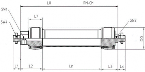
Figure 2 shows a model of a PAM type and dimensions of the fluidic muscle that this study will concentrate on the fluidic muscle (DMSP-20-100N-RM-CM) from the FESTO Company. Because it responds more quickly than other types and movements like a natural muscle, its work efficiency is up to 50% closer to the biological muscles. Theoretical Fluidic Muscle force at maximum operating pressure is 1500N, the mode of operation is single-acting mode and pulling mode, and the maximum working load freely suspended is 80Kg. The operating pressure of this kind is between 0 MPa and 0.6 MPa [25].
Figure 2 shows the two dimensions (2D) of the fluidic muscle type DMSP-20-100N-RM-CM. Also, Table 1 illustrated the values of the dimensions.
Some of the values that affected the performance and considered as a limitation in this type of artificial muscle and affect the control results. The stroke of the muscle max. value is 2500 mm, and the operating pressure is from 0 bar to 6 bar, giving force at the maximum pressure is 1500 N, and the max working load freely suspended is 80 Kg.
Before forming the design control first order develop a mathematical model of the system that accurately echoes real muscle behavior. The PAM system is able to be examined and its connected controller is designed to suit the performance requirements.
Figure 2. Dimensions of the fluidic muscle type DMSP-20-100N-RM-CM [25]
Table 1. Dimensions values [25]
|
Dimensions |
value |
|
SW1 |
17mm |
|
SW2 |
10mm |
|
SW4 |
13mm |
|
L1 |
15mm |
|
L2 |
36mm |
|
L3 |
26mm |
|
L4 |
15mm |
|
L7 |
19mm |
|
L8 |
142mm |
|
LN |
80mm |
|
DO |
22mm |
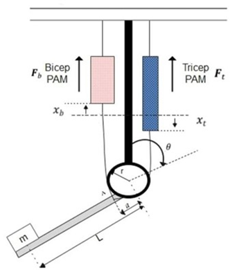
Figure 3. PAM single-link robot arm
Figure 3 shows a mass with PAMs actuated by arm positions of the triceps and biceps. The wrist moves as the PAMs expand and compress while the upper arm stays fixed. The upper arms and endpoints of the PMs are attached to a fixed reference point. where m denotes mass in (kg), g represents gravitational acceleration (m/s2), r is the pulley radius (m), xt represents pneumatic muscle extension (m), and xb is the muscle contraction (m). The PMs are attached to the elbow at point A, which is a rotational axis away from the joint. L is distance between joint and the load's center of mass.
The amount of pneumatic muscle extension xt and muscle contraction xb can be expressed respectively by researches [26, 27]:
$x_b=a(1-\cos \theta)$ (1)
$x_t=a(1+\cos\theta)$ (2)
The movement of the wrist shown an angle α=sin-1 (r/a) with the triceps corps. Within the same angle θ, the wrist is authorized to twist. The angle θ=0 corresponds to the wrist in a descending position, whereas angle θ=π represents a case that the wrist is positioned extremely upwards. The wrist's biceps muscle produces a clock - wise torque that is provided by research [28]:
$\tau_{c w}= F_b(\cdot) \ a \ \sin \theta$ (3)
The counterclockwise torque applied by the triceps muscle is described by:
$\tau_{c c w}=\ F_t(.) \ r$ (4)
In this equation, Ft(.) and Fb(.) represent the forces produced by the triceps and bicep muscles of the PAMs, respectively, and r is the radius of the pulley. These forces can be described by the dynamic PAM model:
$F_b(.)=F\left(P_b\right)-K\left(P_b\right) x_b-B\left(P_b\right) x_b$ (5)
$F_t(.)=F\left(P_t\right)-K\left(P_t\right) x_t-B\left(P_t\right) x_t$ (6)
In this equation, B(Pt) B(Pb) represents the bicep muscle's coefficient of viscous friction, L is the distance between the mass's centroid and the joint, B(Pt) represents the tricep muscle's coefficient of viscous friction, K(Pb) denotes the bicep muscle's spring coefficient (in units of Newtons per meter), K(Pt) denotes the tricep muscle's spring coefficient (in units of Newtons per meter). F(Pb), represents the force exerted by the PAM in the bicep case, and F(Pt) represents the force exerted by the PAM in the tricep case. The variable 'a' represents the distance between the joint axis of rotation and the PAM's attachment point. The variables F(Pb), K(Pb), and B(Pb) represent the bicep PAM's force, spring coefficient, and viscosity coefficient, respectively, and they can be expressed in the following form:
$\left.\begin{array}{c}F\left(P_b\right)=F_b+F_1 P_b \\ K\left(P_b\right)=K_b+K_1 P_b \\ B\left(P_b\right)=B_{0 b}+B_{1 b} P_b\end{array}\right\}$ (7)
As well, F(Pt), K(Pt), and B(Pt) characterize triceps of the PAM force, spring, and viscosity coefficients, so that the associated formulas explain them:
$\left.\begin{array}{c}F\left(P_t\right)=F_t+F_1 P_t \\ K\left(P_t\right)=K_t+K_1 P_t \\ B\left(P_t\right)=B_{0 t}+B_{1 t} P_t\end{array}\right\}$ (8)
It is important to point out that coefficient B relies on whether a muscle is already in compressed mode or stretched mode, which is, one has varied coefficients of the triceps and bicep B(Pt) and B(Pb). Therefore, by combining the torques described by Eq. (3) and Eq. (4), one can find the dynamics motion equation:
$\ddot{I} \theta=F_b(.) a \sin \theta-F_t(.) r-M g L \sin \theta$ (9)
where, I=ML2 describes the moment of mass inertia about the elbow and the latest term (M*g*L*sinθ) has been adjusted to take into consideration the mass gravity's counterclockwise torque on the forearm. So can achieve the following by substituting Eqns. (5) and (6) into Eq. (9):
$\begin{aligned} I \ddot{\theta}=n\left(F\left(P_b\right)-\right. & \left.K\left(P_b\right) x_b-B_b\left(P_b\right) \dot{x}_b\right) a \sin \theta \\ & -\left(F\left(P_t\right)-K\left(P_t\right) x_t\right. \\ & \left.-B_t\left(P_t\right) \dot{x}_t\right) r-M g L \sin \theta\end{aligned}$ (10)
The time derivative of PM extension xt and contraction xb are given, respectively, as:
$\dot{x}_b=a(\sin \theta) \dot{\theta}$ (11)
$\dot{x}_t=-a(\sin \theta) \dot{\theta}$ (12)
Using Eqns. (10) and (12), one can get:
$\begin{aligned} I \ddot{\theta}=n\left(F\left(P_b\right)-\right. & \left.K\left(P_b\right) x_b-B_b\left(P_b\right) \ \dot{x}_b\right) a \sin \theta \\ & -\left(F\left(P_t\right)-K\left(P_t\right) x_t-B_t\left(P_t\right) \dot{x}_t\right) \\ & -M g L \sin \theta\end{aligned}$ (13)
The pressure of triceps and biceps PAM is given:
$P_b=P_{o b}+\Delta P$ (14)
$P_t=P_{o t}-\Delta P$ (15)
where, P0t, and P0b represent primary pressure of triceps and biceps, respectively, ∆P is designated as system's control input, and it displays how much pressure exists between both the triceps and biceps. Then combined the Eq. (14 and 16), to produce:
$\begin{aligned} I \ddot{\theta}=\left[\left(a F_0+a F_1\right.\right. & \left.P_{0 b}-M g L\right) \sin \theta \\ & +a^2\left(K_0+K_1 P_{0 b}\right) \sin \theta(\cos \theta \\ & -1)-a^2\left(B_{0 b}+B_{1 b} P_{0 b}\right) \sin ^2 \theta . \dot{\theta} \\ & +a r\left(K_0+K_1 P_{0 t}\right) (1+\cos \theta) \\ & -a r\left(B_{0 t}+B_{1 t} P_{0 t}\right) \sin \theta \cdot \dot{\theta} \\ & \left.-r\left(F_0+F_1 P_{0 t}\right)\right]+\left[a F_1 \sin \theta\right. \\ & +a^2 K_1 \sin \theta(\cos \theta-1) \\ & -a^2 B_{1 b} \sin ^2 \theta . \dot{\theta} \\ & -a r K_1(1+\cos \theta) \\ & \left.+a r B_{1 t} \sin \theta . \dot{\theta}+r F_1\right] \Delta P\end{aligned}$ (16)
where, Eq. (16) can be rewritten in the following compact form:
$\ddot{\theta}=f(\theta, \dot{\theta})+b(\theta, \dot{\theta}) \Delta P$ (17)
where is $f(\theta, \dot{\theta})$ and $b(\theta, \dot{\theta})$ are defined by:
$f(\theta, \dot{\theta})=\sum_1^6 f_i Z_i(\theta, \dot{\theta})$ (18)
$b(\theta, \dot{\theta})=\sum_1^6 b_i Z_i(\theta, \dot{\theta})$ (19)
where, i = 1, 2, · ·, 6. The classification of coefficients' factors fi, Zi and bi have been listed in Table 2. The difference between the pressures is the ∆P and given in Eq. (14) is characterized as a control signal; that is u = ∆P. additionally, if state variable $x_1$ is assigned to angular position θ and state variable x2 denotes angular velocity θ, then the following describes a state space representation: Eq. (20) [29]:
$\begin{gathered}x_1=\theta, \dot{x}_1=\dot{\theta}=x_2 \\ \dot{x}_2=\ddot{\theta}=\ddot{x}_1=f(\theta, \dot{\theta})+b(\theta, \dot{\theta}) u \\ =f\left(x_1, x_2\right)+b\left(x_1, x_2\right) u\end{gathered}$ (20)
Figure 4 presents the MATLAB/SIMULINK /R2019a for the PAM actuated arm. The simulation of PAM actuated arm, the model representation is by using Eq. (20). Table 3 displays the values of the PAM model's actuated arm variables that were used in the simulations. These variables cause the non-linearities and the instabilities that shown in the results of the open loop.
Table 2. Classifications of the coefficient factors fi, Zi and bi
|
Zi |
fi |
bi |
|
$z_1=\sin x_1$ |
$\begin{aligned} & f_1 \\ &=\left(a F_0+a F_1 P_{0 b}\right. \\ &-M g L) / I\end{aligned}$ |
$b_1=a F_1 / I$ |
|
$\begin{aligned} & \quad z_2 \\ & =\sin x_1\left(\cos x_1\right. \\ & -1)\end{aligned}$ |
$f_2=a^2\left(k o+K_1 P_{o b}\right) / I$ |
$b_2=a^2 K_1 / I$ |
|
$z_3=\left(\sin ^2 x_1\right) \ x_2$ |
$f_3=-a^2\left(B_{0 b}+B_{1 b} P_{o b}\right)/ I$ |
$\begin{gathered}b_3 =-a^2 B_{1 b} / I\end{gathered}$ |
|
$z_4=1+\cos x_1$ |
$f_4=\operatorname{ar}\left(k o+K_1 P_{0 t}\right) / I$ |
$\begin{gathered}b_4 =-\operatorname{ar} K_1 / I\end{gathered}$ |
|
$z_5=\left(\sin x_1\right) x_2$ |
$f_5=-\operatorname{ar}\left(B_{0 t}+B_{1 t} P_{0 t}\right)/ I$ |
$\begin{gathered}b_4=-a r K_1 / I\end{gathered}$ |
|
$z_6=1$ |
$f_6=\left(-r F_0-r F_1 P_{0 t}\right) / I$ |
$b_6=r F_1 / I$ |
Figure 4. Open loop PAM manipulator arm system represented by MATLAB SIMULINK
Table 3. The mathematical values of the coefficient of the PAM
|
Coefficient descriptions |
Values |
|
The nominal force that has been exerted by PAM (F0) |
0.986×10²N |
|
Variation in a force exerted by PAM (F1) |
0.803N |
|
variation in the coefficient of viscosity in the bicep muscle (B1b) |
4.66x10⁻³N.s/m |
|
Bicep /nominal viscosity coefficient (B0b) |
1.35N.s/m |
|
Standard spring coefficient (k0) |
6.51N/m |
|
Triceps /nominal viscosity Coefficient (B0t) |
4.03x10⁻¹N.s/m |
|
Triceps /variation in viscosity coefficient (B1t) |
12.0x10⁻⁴N.s/m |
|
Nominal bicep pressure (Pob) |
510.4KPa |
|
Variation in spring coefficient (k1) |
2.12×10⁻²N/m |
|
The distance of the mass center from the joint (L) |
0.46m |
|
Nominal triceps pressure (Pot) |
400Pa |
|
Mass (M) |
20kg |
|
Pulley radius (r) |
0.0508m |
|
Distance between the PAM attachment point and the joint axis (a) |
0.0762m |
|
Gravity Acceleration (g) |
9.8m/s2 |
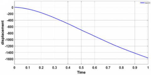
Both controllers that apply to the system are applied in MATLAB/SIMULINK software and was used to create the models. The results of the open loop position and velocity are shown in Figure 5. Using the Backstepping Control (BSC) then apply the Adaptive Backstepping Control (ABSC) on the PAM's arm manipulator model to solve the main problem and to stabilize the PAM and transfer its states to the balance point area. The since the main issue of the PAM model is unstable and uncontrollable due to the deficiency of speed control, resulting in unwanted movement that requires to be regulated. Figure 5 shows that the open loop system is unstable.
Table 3 lists the mathematical values for both PAM-actuated Single Arm Manipulators in the bicep/triceps positions [30].
a. Displacement of the single arm actuator
b. Velocity of the single arm actuator
Figure 5. Open loop response of the single arm actuator by using PAM
In this section, we have designed control methods for studying the control design for the PAM robot arm's movement. We developed the control design using a BSC technique [31, 32]. The dynamic responsiveness of the controlled system is directly influenced by the design parameters of the BSC [33]. Establish the BSC algorithm for a Single Arm PAM-Actuated Robot system by following the procedures listed [34].
Let the variation between actual angle position x1=θ and needed trajectory x1d=θd be the e as the follow [35, 36].
The time derivative of the error in Eq. (21), the tracking velocity, can be written as follows:
$e_1=x_1-x_{1 d}$ (21)
Defining the first virtual control α1=x2 and sub in Eq. (22) to get:
$\dot{e_1}=\dot{x}_1-\dot{x}_{1 d}$ (22)
Defining the first virtual control α1=x2 and sub in Eq. (22) to get:
$\dot{e}_1=\alpha_1-\dot{x}_{1 d}$ (23)
The Lyapunov function is a type of function that is always positive, and its derivative is also a function as follows:
$V_1=\frac{1}{2} e_1^2$ (24)
$\dot{V}_1=e_1 \dot{e}_1$ (25)
By substituting Eq. (23) into Eq (25), we can obtain a new derivative of the Lyapunov function, which can be written as follows:
$\dot{V}_1=e_1\left(\alpha_1-\dot{x}_{1 d}\right)$ (26)
A virtual control ( $\alpha_1=-c_1 e_1+\dot{\mathrm{x}}_{1 \mathrm{~d}}$ ) is created and sub into Eq. (26) then:
$\dot{V}_1=-c_1 e^2{ }_1$ (27)
This mean V1< 0 Let the error e2, between actual state x2 and the first virtual control α1 described by Eq. (28) and taking the time derivative of Eq. (28) and using Eq. (20) to get:
$e_2=x_2-\alpha_1$ (28)
$\dot{e_2}=\dot{x}_2-\dot{\alpha}_1$ (29)
$\dot{e}_2=f\left(x_1, x_2\right)+b\left(x_1, x_2\right) u-\dot{\alpha}_1$ (30)
The second Lyapunov function is:
$V_2=\frac{1}{2} e^2{ }_1+\frac{1}{2} e^2{ }_2$ (31)
Using the time derivative of Lyapunov function and the derivative of Lyapunov function leads to:
$\dot{V}_2=e_1 \dot{e}_1+e_2 \dot{e}_2$ (32)
$\dot{V}_2=-c_1 e^2{ }_1+e_2\left(f\left(x_1, x_2\right)+b\left(x_1, x_2\right) u-\dot{\alpha}_1\right)$ (33)
Choosing the control law:
$u=\frac{-c_2 e_2-e_1-f\left(x_1, x_2\right)-c_1 \dot{e}_1+\ddot{x}_{1 d}}{b\left(x_1, x_2\right)}$ (34)
The result of the Lyapunov function's derivative is:
$\dot{V}_2=-c_1 e^2{ }_1-c_2 e^2{ }_2$ (35)
Figure 6 below shows graphical design of BSC for PAM - actuated robot arm and shows the control law that controls t he PAM-actuated robot arm.
3.1 Adaptive backstepping control
Adaptive control can effectively address uncertainty. A backstepping-based adaptive control method is proposed to offer a non-linear recursive technique for monitoring that is based on the precise construction of Lyapunov functions. This approach enables the handling of unknown parameters and nonlinear effects [37].
In this section, ABSC was created to evaluate the disturbance and stabilize the position and angular orientation of the PAM. A parameter estimator, which provides estimations of unknown parameters, and a control rule are used to create an adaptive controller. It can guarantee the asymptotic tracking and boundedness of the closed-loop states [38, 39].
The sequence of equations given below can be used to develop the ABSC algorithm for a PAM system.
Let e be the difference between the actual angle position x1 = θ and the desired trajectory x1d = θd as follows:
$e_1=x_1-x_{1 d}$ (36)
The time derivative of the error in Eq. (36), the tracking velocity, can be written as follows:
$\dot{e}_1=\dot{x}_1-\dot{x}_{1 d}$ (37)
$\dot{e_1}=x_2-\dot{x}_{1 d}$ (38)

Figure 6. Schematic diagram of the proposed BSC for PAM
Defining the first virtual control α1=x2 and sub in Eq. (38) to get:
$\dot{e_1}=\alpha_1-\dot{x}_{1 d}$ (39)
The positive Lyapunov function in Eq. (40) and the Lyapunov function derivative during time is in Eq. (41):
$V_1=\frac{1}{2} e_1^2$ (40)
$\dot{V}_1=e_1 \dot{e_1}$ (41)
As follows: by substituting Eq. (39) into Eq. (41) to generate a new derivative of the Lyapunov function, which can be shown as follows:
$\dot{V}_1=e_1\left(\alpha_1-\dot{x}_{1 d}\right)$ (42)
A virtual control is formed in Eq. (43):
$\alpha_1=-c_1 e_1+\dot{x}_{1 d}$ (43)
Sub Eq. (43) into Eq. (42) to get:
$\dot{V}_1=-c_1 e_1^2$ (44)
Tacking the time derivative of the virtual control:
$\dot{\alpha}_1=-c_1 \dot{e}_1+\ddot{x}_{1 d}$ (45)
Sub Eq. (38) into the Equation of the time derivative of the virtual control:
$\dot{\alpha}_1=-c_1 x_2+c_1 \dot{x}_{d 1}+\ddot{x}_{1 d}$ (46)
By tacking the e2 as a tracking error, between actual state x2 and the first virtual control α1 described by Eq. (47) and then taking the time derivative of Eq. (47).
$e_2=x_2-\alpha_1$ (47)
$\dot{e_2}=\dot{x_2}-\dot{\alpha_1}$ (48)
and using Eq. (20) to get:
$\dot{e_2}=f\left(x_1, x_2\right)+b\left(x_1, x_2\right) u-F_{d 1}-\dot{\alpha}_1$ (49)
$\begin{aligned} \dot{e}_2=f\left(x_1, x_2\right)+ & b\left(x_1, x_2\right) u-F_{d 1}+c_1 x_2-c_1 \dot{x}_{1 d} -\ddot{x}_{1 d}\end{aligned}$ (50)
Fd1 is supposed to be unknown external disturbance.
The second Lyapunov function is:
$V_2=\frac{1}{2} e_1^2+\frac{1}{2} e_2^2+\frac{1}{2} \gamma_1^{-1} \tilde{F}_{d 1}^2$ (51)
Using the time derivative of Lyapunov function, where the $\tilde{F}_1$ represents the estimation error disturbance:
$\tilde{F}_{d 1}=F_{d 1}-\hat{F}_{d 1}$ (52)
$\widehat{F}_{d 1}$ the estimation of disturbance Fd1 denoted.
Tacking the time derivative of estimation error disturbance
$\dot{\tilde{F}}_{d 1}=-\dot{\hat{F}}_{d 1}$ (53)
Taking the derivation of equation V2 with respect of time:
$\dot{V}_2=e_1 \dot{e}_1+e_2 \dot{e}_2+\gamma_1^{-1} \tilde{F}_{d 1} \dot{\tilde{F}}_{d 1}$ (54)
$\dot{V}_2=-c_1 e^2{ }_1+e_2\left(f\left(x_1, x_2\right)+b\left(x_1, x_2\right) u-\dot{\alpha}_1\right)$ (55)
Choosing the control law:
$u=\frac{-c_1 x_2-e_1-c_2 e_2-f\left(x_1, x_2\right)+c_1 \dot{x}_{1 d}+\ddot{x}_{1 d}-\hat{F}_{d 1}}{b\left(x_1, x_2\right)}$ (56)
from Eq. (56) and Eq. (55) and estimation error disturbance:
$\dot{V}_2=e_1 \dot{e}_1+e_2 \dot{e}_2+\gamma_1^{-1} \tilde{F}_{d 1} \dot{\tilde{F}}_{d 1}$ (57)
The derivative of Lyapunov function leads to:
$\dot{\hat{F}}_1=\gamma_1 e_2$ (58)
Using the first update adaptive law into Eq. (56) gives:
$\dot{V}_2=-c_1 e_1^2-c_2 e_2^2$ (59)
This section represents a comparison between BSC and ABSC for single-arm PAM-actuated robot stabilization, tracking, and regulatory control. Using MATLAB/SIMULINK/2019a simulation to investigate the BSC and ABSC implementation and evaluate the controllers. The coefficient values affecting the system for a single-arm PAM-actuated robot are illustrated in Table 3. both controllers based on the try-and-error approach in Table 4. includes the controller design parameter's using the method that relies on determining values through trial and error.
Table 4. Factors that influence control design values
|
Factors |
BSC |
ABSC |
|
C1 |
1 |
26 |
|
C2 |
1 |
34 |
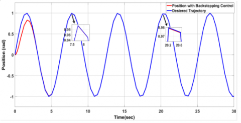
A comparison was accomplished using the response of stability in the position tracking for the PAM-actuated arm moving. As mentioned previously that the BSC algorithm requires validation as well. The comparison has been performed with the use of position tracking in the valve during PAM-actuated arm moving. The time response for PAM actuated arm moving was obtained from the BSC reaching the equilibrium at a stable state at 6 sec. but the response of using the ABSC reaches its steady at 0.2 sec. Backstepping controllers and Adaptive Backstepping controllers based on the try-and-error method.
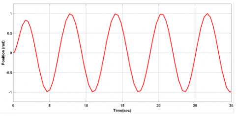
Figures 7 and 8 below shows the position and the velocity control signal using the BSC technique, the position control signal tracking shows that at time 6 sec reaches its steady-state but the signal has chattering and not smooth. The error between the desired signal and the position with non-optimal BSC is 5*10-4. The Simulink of the ABSC in MATLAB/2019/b simulation shown in Figure 9.
Figure 7. Position trajectory of the BSC
Figure 8. Velocity trajectory of the BSC
Figure 9. PAM manipulator arm system controlled by ABSC represented by MATLAB SIMULINK
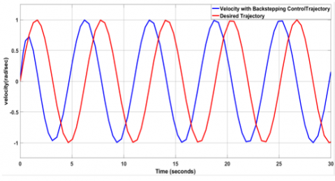
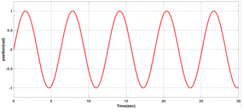
The position and velocity control signal using the ABSC method the position control signal tracking shows in Figures 10 and 11 that at time 0.2 sec reaches its steady-state the signal has been smoother and almost there is no chattering in it. The error between the desired signal and the position with ABSC is 9.985*10-6.
Figures 12 and 13 show the compared signal between the BSC and ABSC that the desire to achieve obviously indicates that the signal of utilizing the ABSC is more accurate and less chattering this is cause precise performance and smoother movement.
Figure 10. Position trajectory of the ABSC
Figure 11. Velocity trajectory of the ABSC
Figure 12. Position BSC signal
Figure 13. Position ABSC signal
Through using the backstepping method to control movement, a PAM actuator arm is developed and implemented in this research. The controller is then modified into an adaptive Backstepping controller for the PAM actuator arm. Furthermore, a comparison between the two controllers was developed. It turns out that the law of control is what precisely enables the arm manipulator's movements to follow the required trajectory. throughout the control diagram simulation in MATLAB/2019/b. BSC and ABSC controllers are developed using the trial-and-error method of fine-tuning, which leads to the finding of positive constants. The comparison showed that using ABSC reduces error, improves accuracy, and produces output signals with little chatter. As compared to the response in the PAM actuated the arm model in the current study utilizing the ABS controller system revealed a fair enhancement in the error lowering by 98% from the BS controller system. It has been proven that an Adaptive backstepping controller can control the uncertainties, and the chattering in the output signal and maintain the controlled system’s stability.
The error in the BSC is also small but the accuracy and reaching the stability is more than the ABSC, however, the signal inaccuracy and chatter are excessive and have inaccurate consequences on the motion performance and the exact position of the PAM actuation arm. The ABSC has been demonstrated to be more capable of dealing with perturbations and uncertainty. To ensure precise results and strong performance, next work will utilize optimization methods to fine-tune the controller parameters.
[1] Khames, L., Al-Jodah, A. (2018). Second order sliding mode controller design for pneumatic artificial muscle. Journal of Engineering, 24(1): 159-172.
[2] Bravo, R.R.S., De Negri, V.J., Oliveira, A.A.M. (2018). Design and analysis of a parallel hydraulic–pneumatic regenerative braking system for heavy-duty hybrid vehicles. Applied Energy, 225: 60-77. https://doi.org/10.1016/j.apenergy.2018.04.102
[3] Azlan, N.Z., Kamarudzaman, N. (2021). Soft pneumatic exoskeleton for wrist and thumb rehabilitation. International Journal of Robotics and Control Systems, 1(4): 440-452. https://doi.org/10.31763/ijrcs.v1i4.447
[4] Reynolds, D., Repperger, D., Phillips, C., Bandry, G. (2003). Modeling the dynamic characteristics of pneumatic muscle. Annals of Biomedical Engineering, 31: 310-317. https://doi.org/10.1114/1.1554921
[5] Repperger, D.W., Johnson, K.R., Phillips, C.A. (1998). A VSC position tracking system involving a large scale pneumatic muscle actuator. In Proceedings of the 37th IEEE Conference on Decision and Control (Cat. No. 98CH36171), Tampa, FL, USA, pp. 4302-4307. https://doi.org/10.1109/CDC.1998.761982
[6] Humaidi, A.J., Kadhim, S.K., Sadiq, M.E., Abbas, S.J., Al-Dujaili, A.Q., Ajel, A.R. (2022). Design of optimal sliding mode control of pam-actuated hanging mass. ICIC Express Letters, 16(11): 1193-1204. https://doi.org/10.24507/icicel.16.11.1193
[7] Karnjanaparichat, T., Pongvuthithum, R. (2008). Adaptive control for a one-link robot arm actuated by pneumatic muscles. Chiang Mai Journal of Science, 35(3): 437-446.
[8] Robinson, R.M., Kothera, C.S., Wereley, N.M. (2014). Variable recruitment testing of pneumatic artificial muscles for robotic manipulators. IEEE/asme Transactions on Mechatronics, 20(4): 1642-1652. https://doi.org/10.1109/TMECH.2014.2341660
[9] Ahmed, A.S., Kadhim, S.K. (2022). A Comparative Study Between Convolution and Optimal Backstepping Controller for Single Arm Pneumatic Artificial Muscles. Journal of Robotics and Control (JRC), 3(6): 769-778. https://doi.org/10.18196/jrc.v3i6.16064
[10] Sadiq, M.E., Humaidi, A.J., Kadhim, S.K., Al Mhdawi, A., Alkhayyat, A., Ibraheem, I.K. (2021). Optimal Sliding Mode Control of Single Arm PAM-Actuated Manipulator. In 2021 IEEE 11th International Conference on System Engineering and Technology (ICSET), Shah Alam, Malaysia, pp. 84-89. https://doi.org/10.1109/ICSET53708.2021.9612539
[11] Šitum, Ž., Trslić, P., Trivić, D., Štahan, V., Brezak, H., Sremić, D. (2015). Pneumatic muscle actuators within robotic and mechatronic systems. In Proceedings of International Conference Fluid Power, Fluidna tehnika 2015, pp. 175-188.
[12] Isidori, A. (2013). Nonlinear control systems II. Springer London. https://doi.org/10.1007/978-1-4471-0549-7
[13] Sastry, S. (2013). Nonlinear Systems: Analysis, Stability, and Control (Vol. 10). Springer Science & Business Media. https://doi.org/10.1007/978-1-4757-3108-8
[14] Hassan, T., Cianchetti, M., Moatamedi, M., Mazzolai, B., Laschi, C., Dario, P. (2018). Finite-element modeling and design of a pneumatic braided muscle actuator with multifunctional capabilities. IEEE/ASME Transactions on Mechatronics, 24(1): 109-119. https://doi.org/10.1109/TMECH.2018.2877125
[15] Zhang, L., Xie, J., Lu, D. (2007). Adaptive robust control of one-link joint actuated by pneumatic artificial muscles. In 2007 1st International Conference on Bioinformatics and Biomedical Engineering, Wuhan, China, pp. 1185-1189. https://doi.org/10.1109/ICBBE.2007.306
[16] Ba, D.X., Ahn, K.K. (2018). A robust time-delay nonlinear controller for a pneumatic artificial muscle. International Journal of Precision Engineering and Manufacturing, 19: 23-30. https://doi.org/10.1007/s12541-018-0003-5
[17] Tomori, H., Hiyoshi, K. (2018). Control of pneumatic artificial muscles using local cyclic inputs and genetic algorithm. In Actuators, 7(3): 36. https://doi.org/10.3390/act7030036
[18] Caldwell, D.G., Medrano-Cerda, G.A., Goodwin, M. (1995). Control of pneumatic muscle actuators. IEEE Control Systems Magazine, 15(1): 40-48. https://doi.org/10.1109/37.341863
[19] Jahanabadi, H., Mailah, M., Md Zain, M.Z., Hooi, H.M. (2011). Active force with fuzzy logic control of a two-link arm driven by pneumatic artificial muscles. Journal of Bionic Engineering, 8(4): 474-484. https://doi.org/10.1016/S1672-6529(11)60053-X
[20] Chou, C.P., Hannaford, B. (1996). Measurement and modeling of McKibben pneumatic artificial muscles. IEEE Transactions on Robotics and Automation, 12(1): 90-102. https://doi.org/10.1109/70.481753
[21] Chou, C.P., Hannaford, B. (1994). Static and dynamic characteristics of McKibben pneumatic artificial muscles. In Proceedings of the 1994 IEEE International Conference on Robotics and Automation, San Diego, CA, USA, pp. 281-286. https://doi.org/10.1109/ROBOT.1994.350977
[22] Tondu, B., Lopez, P. (2000). Modeling and control of McKibben artificial muscle robot actuators. IEEE Control Systems Magazine, 20(2): 15-38. https://doi.org/10.1109/37.833638
[23] Serres, J.L., Reynolds, D.B., Phillips, C.A., Gerschutz, M.J., Repperger, D.W. (2009). Characterisation of a phenomenological model for commercial pneumatic muscle actuators. Computer Methods in Biomechanics and Biomedical Engineering, 12(4): 423-430. https://doi.org/10.1080/10255840802654327
[24] Reynolds, D., Repperger, D., Phillips, C., Bandry, G. (2003). Modeling the dynamic characteristics of pneumatic muscle. Annals of Biomedical Engineering, 31: 310-317. https://doi.org/10.1114/1.1554921
[25] Users guide of FESTO Company. https://www.festo.com/us/en/c/products/industrial-automation/actuators-and-drives/pneumatic-cylinders/diaphragm-actuators/pneumatic-muscle-id_pim397/, accessed on Aug. 12, 2022.
[26] Lilly, J.H. (2003). Adaptive tracking for pneumatic muscle actuators in bicep and tricep configurations. IEEE Transactions on Neural Systems and Rehabilitation Engineering, 11(3): 333-339. https://doi.org/10.1109/TNSRE.2003.816870
[27] Ahmed, A.S., Saleem, K., Kadhim, S.K. (2022). A comparative study between convolution and optimal backstepping, controller for single arm pneumatic artificial muscles. Journal of Robotics and Control (JRC), 3(6): 769-778. http://dx.doi.org/10.18196/jrc.v3i6.16064
[28] Yang, L., Lilly, J. H. (2003). Sliding mode tracking for pneumatic muscle actuators in bicep/tricep pair configuration. In Proceedings of the 2003 American Control Conference, 2003, Denver, CO, USA, pp. 4669-4674). IEEE. https://doi.org/10.1109/ACC.2003.1242460
[29] Humaidi, A.J., Kadhim, S.K., Gataa, A.S. (2022). Optimal adaptive magnetic suspension control of rotary impeller for artificial heart pump. Cybernetics and Systems, 53(1): 141-167. https://doi.org/10.1080/01969722.2021.2008686
[30] Humaidi, A.J., Ibraheem, I.K., Azar, A.T., Sadiq, M.E. (2020). A new adaptive synergetic control design for single link robot arm actuated by pneumatic muscles. Entropy, 22(7): 723. https://doi.org/10.3390/e22070723
[31] AL-Samarraie, S.A., Abbas, Y.K. (2012). Design of a nonlinear speed controller for a DC motor system with unknown external torque based on backstepping approach. Iraqi Journal of Computers, Communications and Control & Systems Engineering, 12(1): 1-19.
[32] Mohammad, A.M., AL-Samarraie, S.A. (2020). Robust controller design for flexible joint based on back-stepping approach. Iraqi Journal of Computers, Communications, Control and Systems Engineering, 20(2): 58-73. https://doi.org/10.33103/uot.ijccce.20.2.7
[33] Humaidi, A.J., Kadhim, S.K., Gataa, A.S. (2020). Development of a novel optimal backstepping control algorithm of magnetic impeller-bearing system for artificial heart ventricle pump. Cybernetics and Systems, 51(4): 521-541. https://doi.org/10.1080/01969722.2020.1758467
[34] Ma'arif, A., Vera, M.A.M., Mahmoud, M.S., Ladaci, S., Çakan, A., Parada, J.N. (2022). Backstepping sliding mode control for inverted pendulum system with disturbance and parameter uncertainty. Journal of Robotics and Control (JRC), 3(1): 86-92. https://doi.org/10.18196/jrc.v3i1.12739
[35] Salman, M.A., Kadhim, S.K. (2022). Optimal backstepping controller design for prosthetic knee joint. Journal Européen des Systèmes Automatisés, 55(1): 49-59. https://doi.org/10.18280/jesa.550105
[36] Hassan, M.Y., Humaidi, A.J., Hamza, M.K. (2020). On the design of backstepping controller for Acrobot system based on adaptive observer. International Review of Electrical Engineering (IREE), 15(4): 328-335.
[37] Ye, J. (2008). Tracking control for nonholonomic mobile robots: Integrating the analog neural network into the backstepping technique. Neurocomputing, 71(16-18): 3373-3378. https://doi.org/10.1016/j.neucom.2007.11.005
[38] Tohma, D.H., Hamoudi, A.K. (2021). Design of adaptive sliding mode controller for uncertain pendulum system. Engineering and Technology Journal, 39(3): 355-369. https://doi.org/10.30684/etj.v39i3A.1546
[39] Liu, X., Zhang, S., Liu, S., Xu, K., Yao, B. (2020). Adaptive backstepping sliding mode control for a hydraulic knee exoskeleton robot. In 2020 2nd International Conference on Artificial Intelligence, Robotics and Control, pp. 43-48. https://doi.org/10.1145/3448326.3448333