Design of Robust Controller for Nonlinear Systems

Nonlinear systems have been recognized as the most important subject in control field for the previous several decades. They are crucial because of their scientific and engineering applications [1]. Nonlinear phenomena are commonly used to describe the real-world system behavior. Maintaining acceptable stability margins and needed performance parameters in relation to closed-loop systems is difficult because of the substantial nonlinearity and uncertainty of these systems. As a result, robust control approaches are necessary to build nonlinear systems controllers that fulfill the requirements for stability and performance under uncertainty and nonlinearity [2].

A major difficulty in control theory is the construction of strong feedback controllers. These controllers may achieve asymptotically tracking and robustness in the presence of system disturbance and uncertainty [3]. The feedback control theory includes several structure options for feedback as well as various feedback loops. The state feedback control is a sort of feedback control wherein the feedback is accessible for all system states [4]. The H-infinity control, which is considered one of the state feedback control, is the most prevalent and successful method in robust control theory in order to reject a disturbance and compensating uncertainties and nonlinearities in the system. It gives excellent performance and stability [5-8].

Previous studies have concentrated on a range of robust feedback control design methodologies, for example, the development of H-infinity state feedback control depending on a nearly linearized model [9, 10], based on lyapunove theory, the robust feedback linearization for nonlinear process control is built [11], the H-infinity loop - shaping strategy [12, 13], and a robust method of control based on linear & bilinear matrix inequalities, (LMIs) and (BMIs) [14, 15].

Each of the previous research offered somewhat difficult procedure for creating a nonlinear system controller that are particular with relation to the kind of system, which encouraged us to try to use another procedure design method which recommends a simpler and more universal approach.

A proposed full state feedback controller is built in this research to realize the stability for nonlinear systems as well as achieve a desired performance. To determine the best settings for the proposed nonlinear controller, the Black Hole optimization (BHO) approach is utilized. The suggested controller in this study may successfully improve the nonlinear systems behaviour of fixed coefficients.

The rest of this article is organized as following: The black hole optimization (BHO) is detailed in the part "Black Hole Optimization (BHO) method". The concept of the control design based on state feedback control and H-infinity control theory for a nonlinear system is described in the "Controller Design" part. The suggested controller’s parameters that will be adjusted by the (BHO) to get the best values for them were presented in the "Controller Parameters Tuning" part. Two categories of nonlinear systems are offered as case studies in the "Illustrative Examples" part to show the efficacy of the suggested controller. Conclusions are provided in the "Conclusion" section.

This part describes the steps design of suggested controller for systems of the model [20, 21]:

$\begin{gathered}\dot{x}(t)=A x(t)+B_1 d(t)+B_2 u(t) \\ e(t)=C_1 x(t)+D_{12} u(t) \\ y(t)=C_2 x(t)\end{gathered}$                              （3）

where, $x(t) \in \mathcal{R}^n$ represents state vector of the system, $d(t) \in \mathcal{R}^m$ denotes the exogenous disturbance, $u(t) \in \mathcal{R}^l$ depicts the control input, $e(t) \in \mathcal{R}^q$  denotes the controlled output, $y \in \mathcal{R}^p$ represents the output as measured, which is supposed to represent the state vector accessible for feedback, $A \in \mathcal{R}^{n \times n}, B_1 \in \mathcal{R}^{n \times m}$ and $B_2 \in \mathcal{R}^{n \times l}, C_1 \in \mathcal{R}^{q \times n}$ denotes the system state control weight matrix, $D_{12} \in \mathcal{R}^{q \times l}$ represent the control input regulation weight matrix, $C_2 \in \mathcal{R}^{p \times n}$  is aweight matrix of the output.

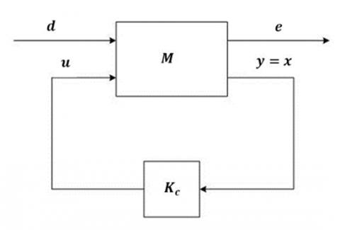
Figure 1 depicts the conventional setup of the complete state feedback H-infinity control, while K_c is the controller gain matrix and M stands for the augmented system matrix [21].

$M=\left[\begin{array}{ccc}A & B_1 & B_2 \\ C_1 & D_{11} & D_{12} \\ C_2 & D_{21} & D_{22}\end{array}\right]$                                  (4)

1.png

Figure 1. The structure of H-infinity full state feedback control

Feedback should be possible for all states of system in order to develop a complete state feedback H-infinity control. This means that C₂=I.D₁₁, D₂₁ and D₂₂ are all equal to zero. As a result, the augmented system matrix M is:

$M=\left[\begin{array}{ccc}A & B_1 & B_2 \\ C_1 & 0 & D_{12} \\ I & 0 & 0\end{array}\right]$                   (5)

The suggested controller design must make the following assumptions:

1. The pairings (A, B₁) & (A, B₂) are supposed to be controllable or, at the very least, stabilizable.

2. The pairing (C₁, A) is supposed to be observable or, at the very least, detectable.

3. $C_1^T D_{12}=0 \& D_{12}^T D_{12}=I$.

It is important to remember that the nonlinear system must be changed to the form described in Eq. (3) utilizing a state variable transformation technique before being controlled in this approach. This transformation arranges nonlinear terms as well uncertainty (bad terms) at the identical channel as the control law u (achieving the matching requirement). In this circumstance, the controller may compensate for the unsatisfactory terms. The diffeomorphism mapping is the suitable transformation for this object:

$\phi: \mathrm{D} \rightarrow \mathcal{R}^n$ this converts the system from x to z space [22].

$z=\phi(x)$                         (6)

The map $\phi$ must be invertable in order to:

$x=\phi^{-1}(z)$                        (7)

The z-space origin point of the modified system equals the point of the initial system [18].

$\phi(0)=0$                             (8)

The above mapping transforms our nonlinear system into the form shown below [9]:

$\dot{z}(t)=A z(t)+B_1 d(t)+B_2 u(t)$                            (9)

The goal of the control challenge is to discover the optimum control law u^*, which is state dependent, that ensures that the closed-loop transfer function’s (T_ed) infinite norm is smaller than a certain value of γ as [20]:

$\left\|T_{e d}(s)\right\|_{\infty}<\gamma$                         (10)

where, γ denotes the upper constraint on the amplitude of the disturbance and perturbation which could be eliminated through the control action. The requirement in Eq. (10) denotes that [21]:

$\underset{u}{\inf} \underset{d}{\sup} J(u, d)<\infty$                         (11)

where,

$J(u, d)=\int_0^{\infty}\left(e^T e-\gamma^2 d^T d\right) d t$                                 (12)

The disturbance d(t) attempts to maximize the cost function J(t), whereas the control signal u(t) intends to minimize it. As a result, the physical connotation of this relationship is that the control action and also the disturbance are in competition with one other within infinmum (inf) and supremum (sup).

Let the structure of the suggested optimal controller and worst-case disturbance be as follows [20]:

$d(t)=K_d x(t)$                            (13)

And

$u(t)=K_c x(t)$                                  (14)

By substituting Eq. (14) into Eq. (3) results in:

$e(t)=\left(C_1+D_{12} k_c\right) x(t)$                                  (15)

Utilising assumption 3, we get:

$e^T e=x^T\left(C_1^T C_1+K_C^T K_c\right) x$                          (16)

Therefore,

$J=\int_0^{\infty} x^T\left(C_1^T C_1+K_c^T K_c-\gamma^2 K_d^T K_d\right) x d t$                                 （17）

Substituting Eqns. (13) and (14) into Eq. (3) results in:

$\dot{x}=\left(A+B_1 K_d+B_2 K_c\right) x$                                    （18）

from the cost function in Eq. (17), can let:

$Q=\left(C_1^T C_1+K_c^T K_c-\gamma^2 K_d^T K_d\right)$                             （19）

where, Q should be positive definite matrix.

By the optimal control law, the system acquired by Eq. (18) is considered to be stable. Based on this assumption, let us develop:

$V(x)=x^T P x$                                                 (20)

$\dot{V}(x)=-x^T Q x$                                  (21)

V(x) represents a Lyapunov function with a positive definite. Eq. (19) would then substituted in Eq. (21) to obtain the best cost function:

$\dot{V}(x)=-x^T\left(C_1^T C_1+K_c^T K_c-\gamma^2 K_d^T K_d\right) x$                                       (22)

$x^T\left(C_1^T C_1+K_c^T K_c-\gamma^2 K_d^T K_d\right) x=-\frac{d}{d t} x^T P x$                                    (23)                

By integrating on each side of Eq. (23) from 0 to $\infty$ gives:

$\begin{gathered}\int_0^{\infty} x^T\left(C_1^T C_1+K_c^T K_c-\gamma^2 K_d^T K_d\right) x d t= \\ \int_0^{\infty}-\frac{d}{d t} x^T P x d t\end{gathered}$                    (24)

$J=-x(\infty)^T P x(\infty)-\left(-x(0)^T P x(0)\right)$                                  (25)

Because the system in Eq. (18) should be stable according to the control law, x(∞)=0. As a result, the optimal cost function is:

$J^*=-x(0)^T P x(0)$                                  (26)

The solution to the following Lyapunov equation is represented by the positive definite matrix P:

$\begin{gathered}\left(A+B_1 K_d+B_2 K_c\right)^T P+P\left(A+B_1 K_d+B_2 K_c\right)=-Q\end{gathered}$                                   （27）

$\begin{array}{r}\left(A+B_1 K_d+B_2 K_c\right)^T P+P\left(A+B_1 K_d+B_2 K_c\right) =-\left(C_1^T C_1+K_c^T K_c-\gamma^2 K_d^T K_d\right)\end{array}$                                       （28）

$\begin{aligned} & \left(A+B_1 K_d+B_2 K_c\right)^T P+P\left(A+B_1 K_d+B_2 K_c\right)  +\left(C_1^T C_1+K_c^T K_c-\gamma^2 K_d^T K_d\right)=0\end{aligned}$                      (29)

To obtain the optimum control law, Eq. (29) must be derived with respect to K_c and set $\partial P / \partial K_{c_{i j}}=0$, we get:

$K_C=-B_2^T P$                                      (30)

As a result,

$u^*=K_c x=-B_2^T P x$                                     (31)

Similarly, we may get the applied worst-case disturbance via deriving the Lyapunov equation with respect to K_d and setting $\partial P / \partial K_{d_{i j}}=0$, we get:

$K_d=\frac{1}{\gamma^2} B_1^T P$                                    (32)

And

$d^*=K_d x=\frac{1}{\gamma^2} B_1^T P x$                                            (33)

And at optimum control condition and worst-case disturbance, we have the Lyapunov equation:

$P A+A^T P+C_1^T C_1-P\left(B_2 B_2^T-\frac{1}{\gamma^2} B_1 B_1^T\right) P=0$                                       (34)

This formula is called H-infinity algebraic riccati equation (HIARE).

The provision $\left\|T_{e d}(s)\right\|_{\infty}<\gamma$ is satisfied and provided:

1. $u^*=K_c x=-B_2^T P x$
2. P>0
3. The matrix A+B₁K_d+B₂K_c is stable, which means that the matrix A+B₂K_c is asymptotically stable as well.

The nonlinear system that must be controlled is:

$\begin{gathered}\dot{x}_1=x_2 \\ \dot{x}_2=\sin x_1-u \times \cos x_1 \\ y=x_1\end{gathered}$                                     (36)

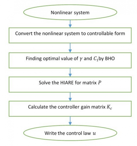
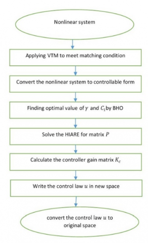
Figure 3 shows the stages of designing the proposed controller for the system described in Eq. (36).

3.png

Figure 3. The controller designing stages for example 1

4.png

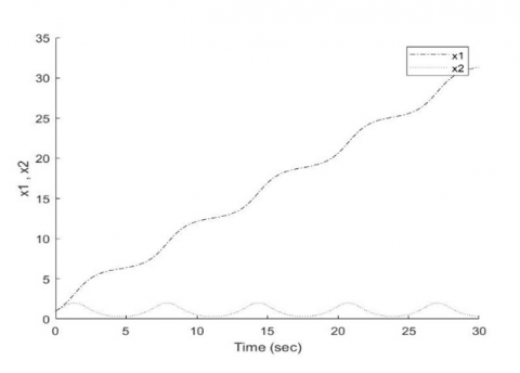
Figure 4. Open-loop system time response prior using the proposed controller

5.png

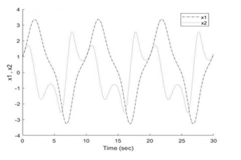
Figure 5. Closed-loop system time response prior using the proposed controller

Figures 4 and 5 depict the open and closed loops nonlinear system time responses features respectively prior to applying the suggested controller. In open-loop, our system is clearly unstable, but in closed-loop, it is critical stable, thus to stabilize the system as well as obtain the desired performance, a controller must be built.

There is no requirement for employ the diffeomophism mapping for this system since all of the nonlinear parts are situated within the same control channel u (the matching condition is met). According to the system equation (Eq. (35)), the factor of u is a nonlinear variable component of the state x₁. As a result, the following procedure is necessary to convert the system equation (Eq. (35)) to the conventional controllable structure as Eq. (3):

$v=-u \times \cos x_1$                            (37)

where, v denotes the virtualized linear state feedback controller, that is:

$v=K_C x=K_1 x_1+K_2 x_2$                                   (38)

Then the actual controller u is:

$u=-\frac{v}{\cos x_1}=-\frac{K_c x}{\cos x_1}=\frac{-K_1 x_1-K_2 x_2}{\cos x_1}$                                         (39)

The state equation for the system that results is:

$\dot{x}(t)=\left[\begin{array}{ll}0 & 1 \\ 0 & 0\end{array}\right] x(t)+\left[\begin{array}{l}0 \\ 1\end{array}\right] d(t)+\left[\begin{array}{l}0 \\ 1\end{array}\right] v(t)$                                 (40)

where,

$d(t)=\sin x_1$                                        (41)

The optimal control law then was determined by using the (BHO) method. Table 1 shows the BHO algorithm optimization setting. Table 2 includes the optimized parameter’s ideal values as well as their limits.

Table 1. The BHO algorithm setting (1st Example)

Table 2. The optimized parameters’ optimal values and bounds (1st Example)

6.png

Figure 6. Stabilization features for the states of the nonlinear system

7.png

Figure 7. (a) Tracking properties of the controlled nonlinear system; (b) x2 behaviour

Following that, the optimal values will be used to solve the H-infinity algebraic riccati problem (Eq. (34)) to get the matrix P of stabilizing positive definiteness as follows:

$P=10^3\left[\begin{array}{ll}0.1843 & 0.0517 \\ 0.0517 & 0.1272\end{array}\right]$                                                     (42)

The state feedback controller’s gain matrix was then calculated using Eq. (30), as shown below:

$K_c=\left[\begin{array}{ll}-51.7 & -127.2\end{array}\right]$                                      (43)

Thus, the control law becomes:

$u=\frac{51.7 x_1+127.2 x_2}{\cos x_1}$                                                     (44)

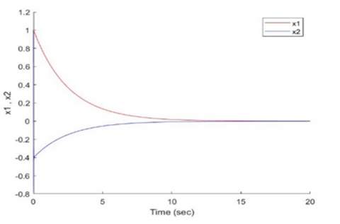
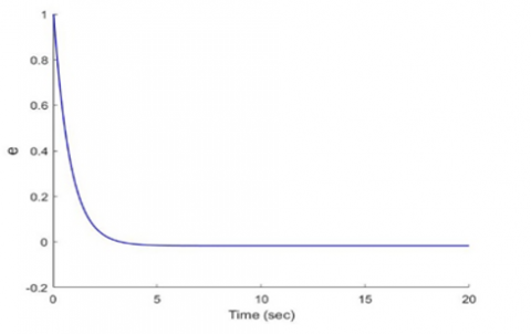
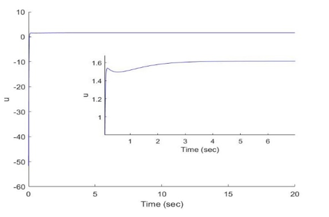
Figure 6 demonstrates the nonlinear system time response behaviour after applying the suggested controller and achieving the stabilization. Figure 7 depicts the output tracking for the entry of a unit step reference and the behaviour of state x₂ which is stable. Figure 8 shows the magnitude of error between input and output signals which is acceptable. Figure 9 depicts the control action behavior. It appears that the suggested controller can successfully stabilizes the nonlinear system while maintaining acceptable performance.

8.png

Figure 8. Error signal properties

9.png

Figure 9. The resultant control action

5.2 Example (2)

Considering the nonlinear system that must be controlled:

$\begin{gathered}\dot{x}_1=\tan x_1+x_2 \\ \dot{x}_2=x_1+u \\ y=x_1\end{gathered}$                                    (45)

Figure 10 shows the stages of designing the proposed controller for the system described in Eq. (45).

10.png

Figure 10. The controller designing stages for example 2

11.png

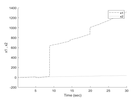
Figure 11. Open-loop system time response prior using the proposed controller

12.png

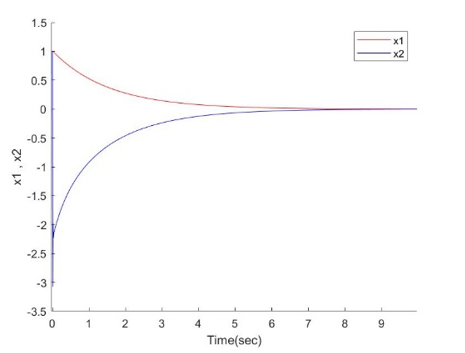
Figure 12. Closed-loop system time response prior using the proposed controller

Figures 11 and 12 depict the open and closed loops nonlinear system time responses features respectively prior to applying the suggested controller.

The system is clearly unstable in both open and closed loops, thus to stabilize the system as well as obtain the desired performance, a controller must be built. Since the nonlinear term (tanx₁) is not placed on the identical channel with the control action u (matching requirement not met), the diffeomorphism mapping for Eq. (6) is required to turn the nonlinear system to its controllable standard structure such as Eq. (9). The state variable transformation shown below is used to carry out the mapping:

$z_1(t)=x_1(t), z_2(t)=\dot{z}_1(t)=\dot{x}_1(t)=\tan x_1+x_2$                                   (46)

Thus, the transformed state equation becomes:

$\begin{gathered}\dot{z}_1(t)=z_2(t) \\ \dot{z}_2(t)=z_1+d(t)+u(t)\end{gathered}$                                               (47)

where,

$d(t)=z_2 \sec ^2 z_1$                                             (48)

The system in z-space then becomes:

$\left[\begin{array}{l}\dot{z}_1(t) \\ \dot{z}_2(t)\end{array}\right]=\left[\begin{array}{ll}0 & 1 \\ 1 & 0\end{array}\right]\left[\begin{array}{l}z_1(t) \\ z_2(t)\end{array}\right]+\left[\begin{array}{l}0 \\ 1\end{array}\right] d(t)+\left[\begin{array}{l}0 \\ 1\end{array}\right] u(t)$                                            (49)

The optimal control law then was determined by using the (BHO) method. Table 3 shows the BHO algorithm optimization setting. Table 4 includes the optimized parameter’s ideal values as well as their bounds.

Table 3. The BHO algorithm settings (2nd Example)

Table 4. The optimized parameters’ optimal values and bounds (2nd Example)

Following that, the optimal values will be used to solve the H-infinity algebraic riccati problem (Eq. (34)) to get the matrix P of stabilizing positive definiteness as follows:

$P=10^3\left[\begin{array}{ll}0.5735 & 0.0823 \\ 0.0823 & 0.1274\end{array}\right]$                                (50)

The state feedback controller’s gain matrix was then calculated using Eq. (30), as shown below:

$K_c=\left[\begin{array}{ll}-82.3554 & -127.4602\end{array}\right]$                                            (51)

As a result, the optimum control law in z-space becomes:

$u=-82.3554 z_1-127.4602 z_2$                                       (52)

The control law is now being transformed from z-space to x-space:

$u=-82.3554 x_1-127.4602 \tan x_1-127.4602 x_2$                                           (53)

13.png

Figure 13. Nonlinear system states’ stabilization qualities

14.png

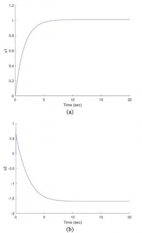
Figure 14. (a) Tracking properties of the controlled nonlinear system; (b) x2 behaviour

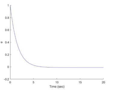
Figures 13 and 14(a) illustrate that, despite the existence of disturbance, the suggested controller succeeded in providing nonlinear system stability and tracking performance efficiency with little tracking error as well as quick converging to the reference input. Figure 14(b) shows the behaviour of state x₂ which is stable. Figure 15 shows the error magnitude between input and output signals which is acceptable. Figure 16 depicts the permissible behavior of the control action that has been executed.

15.png

Figure 15. Error signal properties

16.png

Figure 16. The resultant control action