Mustafa Abdullah*![]() | Hamza Abu Owida
| Hamza Abu Owida![]()
© 2023 IIETA. This article is published by IIETA and is licensed under the CC BY 4.0 license (http://creativecommons.org/licenses/by/4.0/).
OPEN ACCESS
This study employs a theoretical approach to examine the impact of a periodic magnetic field on MHD flow between two infinitely parallel horizontal plates via a porous medium. A periodic magnetic field is imposed in a direction normal to the plates when there is a constant pressure gradient. A periodic flow of heat is used to warm the upper plate, while the lower plate is kept at a constant temperature. To get numerical solutions to the governing partial differential equations, the finite difference approach is employed. Furthermore, an approach known as " Eigen function expansion " is used to solve the equations analytically. Here, we provide a visual depiction and accompanying discussion of the ways in which different variables affect the flow velocity and temperature fields.
magneto hydro dynamics (MHD), porous medium, periodic magnetic field, periodic heat flux, parallel plates
The study of magneto hydrodynamics fluid flow and heat transfer was presented by many researchers in the last decades due to its importance. The MHD study has a wide range of engineering applications in MHD pumps, power generators, cooling systems, the petroleum industry, reactors, accelerators, and many other applications. The influence of no uniform magnetic field, no uniform heat flux and porous medium on the flow and thermal behavior has been studied separately for many systems and many cases.
Several investigations have looked at how a magnetic field affects the flow of a porous material between two parallel plates. In a rotational system with a homogeneous transverse magnetic field, Raju et al. [1] looked at how viscous dissipation and joule heating affected the steady MHD generated convective flow in porous medium down a horizontal channel. It was investigated by Idowu and Olabode [2] how the unsteady MHD flow and heat transfer between infinite parallel porous plates in an inclined magnetic field and a minimal pressure gradient behaves. Ojjela and Naresh [3] studied the two dimensional micropolar fluid flow and heat transfer by magneto hydrodynamics between parallel porous plates. The MHD steady free convection flow with temperature jump at the plates in a vertical parallel plates micro-channel was investigated by Jha et al. [4]. When a heat source and chemical reaction are present in a porous material between two parallel plates impregnated with a porous substance and placed in an oblique magnetic field, the flow of a viscoelastic electrically conducting fluid was studied by Hanvey et al. [5]. In their study, Dwivedi et al. [6] examine how an oblique magnetic field affects the flow of fluid along a horizontal conduit made of porous material. Transient free convection flow of a fluid past an accelerating vertical plate is studied by Abdullah [7] using a theoretical model to examine the effect of magnetic field and periodic wall temperature. Bingham fluid through porous parallel plates has been studied, and the non-linear dimensionless governing equations have been solved numerically [8]. Delhi et al. [9] used transform methods to solve the differential equations to examine the continuous two-dimensional MHD flow between two parallel plates when the plates' angular velocities were different. In their research, Anyanwu et al. [10] looked at the effects of thermal radiation and chemical reactivity on the MHD Couette flow of a fluid between two parallel porous plates. Katagi and Bhat [11] looked into the challenge of maintaining laminar flow in a hydromagnetic field while transporting a viscous, incompressible, electrically conducting fluid between parallel plates. A solution is developed by Ebiwareme et al. [12] for an incompressible fluid bouncing around between two parallel plates at a constant speed.
Prior research had already revealed some findings regarding how MHD flows behave in the absence of a homogeneous magnetic field. The quasielastic magnetic force was examined by Shliomis and Kamiyama [13] as they observed the effects of an oscillating pipe flow in a nonuniform magnetic field. Magnetohydrodynamic flow in an alternating magnetic field was studied by Moreau et al. [14]. An accurate solution to the transient Couette flow in the absence of a homogeneous magnetic field was reported by Asghar and Ahmad [15]. Goharkhah and Ashjaee [16] investigated the impact of a non-uniform magnetic field on a ferrofluid flow with heat transfer via a conduit. In the presence of an alternating magnetic field, the MHD mixed convection of a ferrofluid in a cavity was investigated numerically by Ghaffarpasand [17]. Islam et al. [18] use computational methods to study the free convective heat transfer of a nanofluid in a square enclosure where a non-uniform horizontal magnetic effect predominates.
The influence of periodic wall heat flux on fluid and heat transfer is of great interest in engineering applications, such as the analysis of fluid and heat transfer in heat exchangers and cooling tubes. Magnetohydrodynamic flow through a channel in the presence of heat flux, is studied analytically by Zniber et al. [19]. It is shown that an increase in wall heat flux frequency will improve the average heat transfer between the fluid and the walls at all values of Hartmann number. The influence of sinusoidal wall fluxes on the power-law fluid flowing in concentric circular heat exchanger has been studied by Ho et al. [20]. The temperature distribution and Nusselt numbers were predicted using analytical formulation.
Using a porous medium, this study describes the findings of an examination into the transient convective MHD flow that occurs between two infinitely parallel plates. A combination of a periodic magnetic field perpendicular to the fluid and a periodic wall heat flux with a constant pressure gradient is used to control the fluid's behavior. Numerical solutions to the dimensionless equations are found and then compared to analytical solutions.
The transient laminar incompressible viscous flow in a porous medium between two infinite horizontal plates is considered. A schematic diagram representing the physical model is shown in Figure 1. The plates are separated by a distance d, and rectangular cartesian coordinates are used as shown.
Figure 1. Physical model description
In this paper we studied the influence of a periodic wall heat flux $\frac{\partial T}{\partial y}=-\frac{q}{k} \cos \left(\omega_h^* t^*\right)$ and a periodic magnetic field $B\left(t^*\right)=B_0\left(1+\mathcal{E} \sin \left(\omega_m^* t^*\right)\right)$ with presence of a constant pressure gradient.
At the beginning, the fluid and the plates are stationary and are assumed to have a temperature of T∞. At time t*>0, The lower plate is kept stationary with a constant temperature, while the upper plate in its own plane begins to move with a constant velocity with a periodic heat flux.
By assuming Boussinesq approximation with the presence of a periodic magnetic field, the unsteady momentum and energy governing equations are:
$\frac{\partial u}{\partial t^*}=-\frac{1}{\rho} \frac{\partial p}{\partial x}+g \beta\left(T-T_{\infty}\right)+v \frac{\partial^2 u}{\partial y^2}-\frac{\sigma B_0^2}{\rho}[1+\left.\mathcal{E} \sin \left(\omega_m^* t^*\right)\right] u-\frac{v}{k^*} u$ (1)
$\rho c_p \frac{\partial T}{\partial t^*}=k \frac{\partial^2 T}{\partial y^2}$ (2)
The initial and boundary conditions are:
$\begin{array}{cccl}t^* \leq 0: & u=0 & T=T_{\infty} & \text { for all } y \\ t^*>0: & u=0 & T=T_w & \text { at } y=0 \\ u=u_0 & \frac{\partial T}{\partial y}=-\frac{q}{k} \cos \left(\omega_h^* t^*\right) & \text { at } y=d\end{array}$ (3)
Now the following non-dimensional parameters are introduced:
$X=\frac{x}{d}, Y=\frac{y}{d}, t=\frac{v t^*}{d^2}, \omega_m=\frac{d^2 \omega_m^*}{v}, \omega_h=\frac{d^2 \omega_h^*}{v}, U=\frac{u}{u_0}, \theta=\frac{T-T_{\infty}}{T_w-T_{\infty}}, P=\frac{p d}{u_0 \mu}$, $N=\frac{\sigma d^2 B_0^2}{\mu}, G r=\frac{g \beta d^2\left(T_w-T_{\infty}\right)}{v u_0}, P r=\frac{\mu c_p}{k}, K=\frac{d^2}{k^*}$ (4)
And hence the dimensionless governing equations will be:
$\frac{\partial U}{\partial t}=-\frac{\partial P}{\partial X}+G_r \theta+\frac{\partial^2 U}{\partial Y^2}-[K+N(1+\left.\left.\varepsilon \sin \left(\omega_m t\right)\right)\right] U$ (5)
$\frac{\partial \theta}{\partial t}=\frac{1}{P r} \frac{\partial^2 \theta}{\partial Y^2}$ (6)
With initial and boundary conditions of the form:
$\begin{gathered}t \leq 0: U=0 \quad \theta=0 \quad \text { for all values of } Y \\ t>0: \quad U=0 \quad \theta=1 \quad \text { at } Y=0 \\ U=1 \quad \frac{\partial \theta}{\partial Y}=-\cos \left(\omega_h t\right) \quad \text { at } Y=1\end{gathered}$ (7)
A numerical analysis using the Crank Nicolson technique with the Thomas algorithm is used to solve the dimensionless governing equations. This technique is a fully implicit finite difference method and is hence stable and convergent. It is used to solve a wide range of partial differential equations regarding fluid and heat transfer problems.
The Crank Nicolson finite difference scheme for the dimensionless governing Eq. (6) and Eq. (5) are given by:
$\frac{\theta_i^{n+1}-\theta_i^n}{\Delta t}=\frac{1}{2 P r}\left[\frac{\left(\theta_{i+1}^{n+1}-2 \theta_i^{n+1}+\theta_{i-1}^{n+1}\right)+\left(\theta_{i+1}^n-2 \theta_i^n+\theta_{i-1}^n\right)}{(\Delta Y)^2}\right]$
$\frac{U_i^{n+1}-U_i^n}{\Delta t}=-\frac{\partial P}{\partial X}+G_r \theta_i^{n+1}-[K+N(1+\left.\left.\mathcal{E} \sin \left(\omega_m t\right)\right)\right] U_i^{n+1}+\frac{\left(U_{i+1}^{n+1}-2 U_i^{n+1}+U_{i-1}^{n+1}\right)+\left(U_{i+1}^n-2 U_i^n+U_{i-1}^n\right)}{2(\Delta Y)^2}$
where, i denotes the grid points in the Y direction and n along the time direction.
The above equations can be written in implicit form as:
$\theta_{i-1}^{n+1}-2\left(1+\frac{\operatorname{Pr}(\Delta Y)^2}{\Delta t}\right) \theta_i^{n+1}+\theta_{i+1}^{n+1}=-\theta_{i-1}^n-2\left(\frac{\operatorname{Pr}(\Delta Y)^2}{\Delta t}-1\right) \theta_i^n-\theta_{i+1}^n$
$U_{i-1}^{n+1}-2\left[1+\frac{(\Delta Y)^2}{\Delta t}+\frac{(\Delta Y)^2}{2}\left(K+N\left(1+\varepsilon \sin \left(\omega_m t\right)\right)\right)\right] U_i^{n+1}+U_{i+1}^{n+1}$
$=-U_{i-1}^n-2\left(\frac{(\Delta Y)^2}{\Delta t}-2\right) U_i^n-U_{i+1}^n-2(\Delta Y)^2\left(-\frac{\partial P}{\partial X}+G_r \theta_i^{n+1}\right)$
The above equations with their boundary conditions are considered at every internal point in the y domain forming a tridiagonal system. This system of tridiagonal matrix is solved by applying Thomas algorithm with very small step sizes Δt=0.01 and ΔY=0.001 to ensure accurate results.
An analytical procedure using the Eigen function expansion method is used to validate the numerical solution. Both momentum and energy equations are solved using the same technique, and the results are compared with numerical ones.
4.1 Temperature solution
Firstly the solution of the following dimensionless energy equation will be solved:
$\frac{\partial \theta}{\partial t}=\frac{1}{\operatorname{Pr}} \frac{\partial^2 \theta}{\partial Y^2}$ (8)
With it’s boundary conditions:
$\begin{array}{cc}t \leq 0: \quad \theta=0 \quad \text { for all values of } Y \\ t>0: \quad \theta=1 \quad \text { at } Y=0 \\ \frac{\partial \theta}{\partial Y}=-\cos \left(\omega_h t\right) & \text { at } Y=1\end{array}$ (9)
In order to use the eigenfunction expansion method, the boundary conditions must be linear and homogeneous and hence the following parameter is introduced:
$G(Y, t)=\theta(Y, t)+(Y-1)$ (10)
Thus, the energy equation will be:
$\frac{\partial G}{\partial t}=\frac{1}{\operatorname{Pr}} \frac{\partial^2 G}{\partial Y^2}$ (11)
With the following corresponding boundary conditions:
$\begin{array}{ccc}t \leq 0: & G=Y-1 & \text { for all values of } Y \\ t>0: & G=0 & \text { at } Y=0 \\ \frac{\partial G}{\partial Y}=0 & \text { at } Y=1\end{array}$ (12)
let, G(Y, t)=ψ(Y)δ(t).
Substituting G(Y, t) and it’s derivatives into Eq. (11) and Eq. (12) the eigenvalue problem will be:
$\begin{gathered}\frac{d^2 \psi}{d Y^2}+\lambda \psi=0 \\ \psi(0)=\frac{\partial \psi}{\partial Y}(1)=0\end{gathered}$ (13)
Which have the solution:
$\psi_n(Y)=\sin \left(\sqrt{\lambda_n} Y\right)$ (14)
And the eigenvalues are:
$\lambda_n=\left(\frac{2 n-1}{2} \pi\right)^2$ (15)
The solution for δ(t) is $\delta_n(t)=e^{-\left(\frac{\lambda_n t}{p r}\right)}$.
And then the solution for G(Y, t) is:
$G(Y, t)=\sum_{n=1}^{\infty} B_n \sin \left(\sqrt{\lambda_n} Y\right) e^{\left(\frac{-\lambda_n}{p r} t\right)}$ (16)
Now the initial condition G(Y, 0)=(Y-1) should be applied.
So, the coefficient Bn will be $B_n=\frac{2}{\lambda_n}\left(\sin \sqrt{\lambda_n}-\sqrt{\lambda_n}\right)$, where n=1, 2, ……, ∞.
And the final solution of the dimensionless temperature is:
$\theta(Y, t)=\left(\sum_{n=1}^{\infty} \frac{2}{\lambda_n}\left(\sin \sqrt{\lambda_n}-\sqrt{\lambda_n}\right) \sin \left(\sqrt{\lambda_n} Y\right) e^{\frac{-\lambda_n}{p r} t}\right)+(1-Y)$ (17)
One of the important physical quantities is the local Nusselt number which is given by:
$N u=\frac{-d\left(\frac{\partial T}{\partial y}\right)}{\left(T-T_{\infty}\right)}$ (18)
Hence, according to the temperature solution, the Nusselt number will be:
At the lower plate:
$N u_0=\frac{-1}{\theta(0, t)}\left(\frac{\partial \theta}{\partial Y}\right)_{Y=0}=-\left(\frac{\partial \theta}{\partial Y}\right)_{Y=0}=\left(\sum_{n=1}^{\infty} \frac{2}{\sqrt{\lambda_n}}\left(\sin \sqrt{\lambda_n}-\sqrt{\lambda_n}\right) e^{\frac{-\lambda_n}{p r} t}\right)-1$ (19)
And at the upper plate:
$N u_1=\frac{-1}{\theta(1, t)}\left(\frac{\partial \theta}{\partial Y}\right)_{Y=1}=\frac{1}{\theta(1, t)}$ (20)
4.2 Velocity solution
Using the eigenfunction analytical method, the flow behaviour is computed in the absence of both magnetic field frequency (ωm=0) and Grashof number (Gr=0).
Now let p*=-∂P/∂x the momentum equation will be:
$\frac{\partial U}{\partial t}=p^*+\frac{\partial^2 U}{\partial Y^2}-[K+N] U$ (21)
The boundary conditions are:
$\begin{aligned} & \text { When } t \leq 0: U=0 \quad \text { for all values of } Y \\ & t>0: U=0 \quad \text { at } Y=0 \\ & U=1 \quad \text { at } Y=1 \\ & \end{aligned}$ (22)
Now, the non homogeneous boundary conditions are converted to homogeneous ones by introducing.
$R(Y, t)=\theta(Y, t)-Y$ (23)
Hence the energy equation becomes:
$\frac{\partial R}{\partial t}=\frac{\partial^2 R}{\partial Y^2}-[K+N] R+p^*-[K+N] Y$ (24)
With the following boundary conditions:
$\begin{array}{rlll}\text { When } & t \leq 0: & R=-Y & \text { for all values of } Y \\ & t>0: & R=0 & \text { at } Y=0 \\ & R=0 & \text { at } Y=1\end{array}$ (25)
At the beginning, the following homogeneous part of Eq. (24) will be solved:
$\frac{\partial R}{\partial t}=\frac{\partial^2 R}{\partial Y^2}-[K+N] R$ (26)
By assuming R(Y, t)=α(Y)a(t), the eigenvalue problem will be:
$\begin{gathered}\frac{d^2 \alpha}{d Y^2}+\eta_n \alpha=0 \\ \alpha(0)=\alpha(1)=0\end{gathered}$ (27)
The solution of α(Y) will be:
$\alpha_n(Y)=\sin \left(\sqrt{\eta_n} Y\right)$ (28)
The corresponding eigenvalues are:
$\eta_n=(n \pi)^2$ (29)
And the solution for the time dependent variable a(t) which satisfy the nonhomogeneous Eq. (24) is:
$a_n(t)=\frac{2(-1)^n}{n \pi} e^{-\left(K+N+\eta_n\right) t}+\frac{1}{\left(K+N+\eta_n\right)}\left(\frac{2(-1)^n}{n \pi}\left(K^2+N-\right.\right.\left.\left.p^*\right)+\frac{2 p^*}{n \pi}\right)\left(1-e^{-\left(K+N+\eta_n\right) t\,}\right)$
The series solution of Eq. (26) is:
$R(Y, t)=\sum_{n=1}^{\infty} a_n(t) \sin \left(\sqrt{\eta_n} Y\right)$ (30)
Hence, the final solution will be:
$U(Y, t)=\sum_{n=1}^{\infty} a_n(t) \sin \left(\sqrt{\eta_n} Y\right)+Y$ (31)
The behavior of a viscous incompressible fluid flowing through a porous medium sandwiched between infinite parallel plates is investigated under the influence of a periodic magnetic field and periodic heat flux with a constant pressure gradient. The Crank-Nicolson method is used to numerically solve the governing momentum and energy equations, and the results are checked by solving the problem analytically with a uniform magnetic field and a Grasshoff number of zero.
Graphs display how changing certain variables affects the velocities and temperatures.
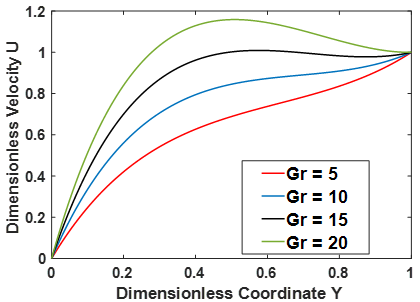
The impact that the Grashof number has on the dimensionless velocity profile is illustrated in Figure 2. It can be observed that the Grashoff number contributes positively to an increase in the fluid's velocity.
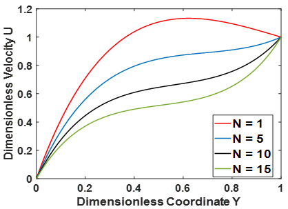
Figure 3 depicts the influence of magnetic field strength, which shows that an increase in the amount of magnetic field strength that is applied creates a delay in the flow.
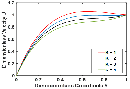
The influence that the permeability parameter has on the velocity profile is shown in Figure 4. It has been observed that increasing K has the effect of slowing down the velocity of the system.
Figure 5 illustrates the effect that the pressure gradient has on the system. It has been noticed that there is a correlation between an increase in the pressure gradient and an enhancement in the fluid's velocity.
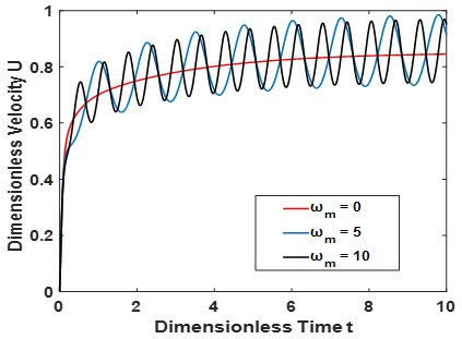
Figures 6 and 7 depict the transient velocity profiles for various fluid locations and magnetic field frequencies, respectively. Figure 6 shows that the velocity grows until it reaches a steady state and that the same periodic pattern of the velocity is observed for different locations of the flow, with the exception that the amplitude increases as one approaches the midpoint between the plates. As shown in Figure 7, the influence of the time-periodic magnetic field on the transient velocity is investigated. Different frequencies are shown to cause the velocity to fluctuate amplitude-wise around a mean value. The velocity behavior appears to have a continuous flow at high frequencies, and the level of fluctuation grows as the magnetic frequency rises.
The effect of the Prandtl number on the temperature field has been shown in Figure 8. It is observed that as the Prandtl number increases, the temperature drops. Also, it can be seen that as we reach steady state behavior, the Prandtl number effect on the temperature becomes less significant as the value decreases.
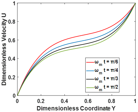
The effect of the magnetic phase angle ωmt on the dimensionless velocity is illustrated in Figure 9. It can be seen that increasing the magnetic phase angle ωmt results in slowing down the fluid velocity U.
Figure 10 illustrates the influence of the heat flow phase angle. It is seen that increasing ωht results in an increase in the fluid temperature $\theta$.
Figure 2. Effect of Grashof number on velocity profile
Figure 3. Effect of magnetic parameter on velocity profile
Figure 4. Effect of permeability parameter on velocity profile
Figure 5. Effect of pressure gradient on velocity profile
Figure 6. Transient velocity at different locations on the Y coordinate
Figure 7. Effect of magnetic frequency on transient velocity
Figure 8. Effect of Prandtl number on temperature profile
Figure 9. Effect of magnetic phase angle ωmt on velocity profile
Figure 10. Effect of heat flux phase angle ωht on temperature profile
Table 1 provides a comparison between the analytical solution and the numerical solution for the transient velocity and temperature in the case of ωm=0 and Gr=0. The results, as shown in the table, are able to be compared with one another and found to be in excellent agreement. This implies that the results found using the Crank Nicolson finite difference method are accurate and can be trusted.
Table 1. Numerical and analytical results for ωm=0 and Gr=0
|
Dimensionless Time |
Dimensionless Velocity |
Dimensionless Time |
Dimensionless Temperature |
||
|
Numerical Value |
Analytical Value |
Numerical Value |
Analytical Value |
||
|
0.1 |
0.3249 |
0.3377 |
1 |
0.2534 |
0.2548 |
|
0.2 |
0.3918 |
0.3938 |
1.5 |
0.3034 |
0.3046 |
|
0.3 |
0.3990 |
0.3990 |
2 |
0.3374 |
0.3384 |
|
0.4 |
0.3997 |
0.3995 |
2.5 |
0.3642 |
0.3651 |
|
0.5 |
0.3998 |
0.3995 |
3 |
0.3863 |
0.3871 |
|
0.6 |
0.3998 |
0.3995 |
3.5 |
0.4048 |
0.4055 |
|
0.7 |
0.3998 |
0.3995 |
4 |
0.4203 |
0.4210 |
Consideration is given to the impact that a periodic magnetic field has on the flow of fluid through a porous medium that is sandwiched between two infinitely parallel plates with a constant pressure gradient and a periodic heat flux. A fully implicit numerical technique is utilized in order to solve the dimensionless governing partial differential equations, and an eigen function expansion method is utilized in order to validate the solution. Graphs illustrating the velocity and temperature profiles along with the effects of a variety of physical parameters are presented. The following are among the findings of the study:
(1) The Grashoff number or the pressure gradient must be increased for there to be an increase in the velocity of the fluid.
(2) A rise in the Prandtl number, the intensity of the magnetic field, or the permeability parameter causes a reduction in the fluid's velocity.
(3) When a periodic magnetic field is used, it is discovered that the transient velocity profile exhibits a periodic pattern of behavior.
(4) An increase in the magnetic phase angle results in flow retardation, while an increase in the heat flow phase angle values contributes to an increase in temperature.
|
B0 |
magnetic flux density, T |
|
Cp |
specific heat, J. kg-1. K-1 |
|
Gr |
Grashof number |
|
k |
thermal conductivity, W.m-1. K-1 |
|
K |
permeability parameter |
|
N |
dimensionless magnetic parameter |
|
p |
pressure, N .m-2 |
|
p* |
dimensionless pressure gradient |
|
P |
dimensionless pressure |
|
Pr |
Prandtl number |
|
q |
heat flux at the wall, W.m-2 |
|
T |
temperature, K |
|
Tw |
wall temperature, K |
|
T∞ |
free stream temperature |
|
t ̃ |
time, s |
|
t |
dimensionless time |
|
u |
velocity, m.s-1 |
|
U |
dimensionless velocity |
|
Nu |
local Nusselt number |
|
X, Y |
dimensionless coordinate |
|
x, y |
Cartesian coordinates, m |
|
Greek symbols |
|
|
α, δ, ψ |
separation variables |
|
Ɵ |
dimensionless temperature |
|
λ, η |
separation constants |
|
$v$ |
kinematic viscosity, m2.s-1 |
|
ρ |
density, kg. m-3 |
|
σ |
electrical conductivity, siemens.m-1 |
|
$\omega_h^*$ |
frequency of heat flux oscillation, rad.s-1 |
|
$\omega_m^*$ |
frequency of magnetic oscillation, rad.s-1 |
|
ωh |
dimensionless frequency of heat flux oscillation |
|
ωm |
dimensionless frequency of magnetic oscillation |
|
B |
dimensionless heat source length |
|
CP |
specific heat, J. kg-1. K-1 |
|
g k |
gravitational acceleration, m.s-2 thermal conductivity, W.m-1. K-1 |
|
Nu |
local Nusselt number along the heat source |
[1] Raju, K.V.S., Reddy, T.S., Raju, M.C., Narayana, P.S., Venkataramana, S. (2014). MHD convective flow through porous medium in a horizontal channel with insulated and impermeable bottom wall in the presence of viscous dissipation and Joule heating. Ain Shams Engineering Journal, 5(2): 543-551. http://dx.doi.org/10.1016/j.asej.2013.10.007
[2] Idowu, A.S., Olabode, J.O. (2014). Unsteady MHD poiseuille flow between two infinite parallel plates in an inclined magnetic field with heat transfer. IOSR Journal of Mathematics, 10(3): 47-53. http://dx.doi.org/10.9790/5728-10324753
[3] Ojjela, O., Naresh, K.N. (2015). Unsteady MHD flow and heat transfer of micropolar fluid in a porous medium between parallel plates. Canadian Journal of Physics, 93(8): 880-887. http://dx.doi.org/10.1139/cjp-2013-0266
[4] Jha, B.K., Aina, B., Ajiya, A.T. (2015). MHD natural convection flow in a vertical parallel plate microchannel. Ain Shams Engineering Journal, 6(1): 289-295. https://doi.org/10.1016/j.asej.2014.09.012
[5] Hanvey, R.R., Khare, R.K., Paul, A. (2017). MHD flow of incompressible fluid through parallel plates in inclined magnetic field having porous medium with heat and mass transfer. IJSIMR, 5(4): 18-22. http://dx.doi.org/10.20431/2347-3142.0504003
[6] Dwivedi, K., Khare, R.K., Paul, A. (2018). MHD Flow through a horizontal channel containing porous medium placed under an inclined magnetic field. Journal of Computer and Mathematical Sciences, 9(8): 1057-1062. http://dx.doi.org/10.29055/jcms/842
[7] Abdullah, M.R. (2018). Transient free convection MHD flow past an accelerated vertical plate with periodic temperature. Chemical Engineering Transactions, 66: 331-336. http://dx.doi.org/10.3303/CET1866056
[8] Mollah, M.T., Islam, M.M., Khatun, S., Alam, M.M. (2019). MHD generalized couette flow and heat transfer on bingham fluid through porous parallel plates. Mathematical Modelling of Engineering Problems, 6(4): 483-490. https://doi.org/10.18280/mmep.060402
[9] Delhi Babu, R., Ganesh, S., Anish, M. (2022). Steady two dimensional MHD stokes flow between two parallel plates under angular velocity with one plate moving uniformly and the other plate at rest and uniform suction at the stationary plate. International Journal of Ambient Energy, 43(1): 741-744. http://dx.doi.org/10.1080/01430750.2019.1672582
[10] Anyanwu, E.O., Olayiwola, R., Shehu, M.D. (2020). Radiative effects on unsteady mhd couette flow through a parallel plate with constant pressure gradient. Asian Research Journal of Mathematic, 1-19. http://dx.doi.org/10.9734/arjom/2020/v16i930216
[11] Katagi, N.N., Bhat, A. (2020). Finite difference solution for MHD flow between two parallel permeable plates with velocity slip. Journal of Advanced Research in Fluid Mechanics and Thermal Sciences, 76(3): 38-48. https://doi.org/10.37934/arfmts.76.3.3848
[12] Ebiwareme, L., Kormane, F.A.P., Odok, E.O. (2022). Simulation of unsteady MHD flow of incompressible fluid between two parallel plates using Laplace-Adomian decomposition method. World Journal of Advanced Research and Reviews, 14(3): 136-145. https://doi.org/10.30574/wjarr.2022.14.3.0456
[13] Shliomis, M.I., Kamiyama, S. (1995). Hydrostatics and oscillatory flows of magnetic fluid under a nonuniform magnetic field. Physics of Fluids, 7(10): 2428-2434. http://dx.doi.org/10.1063/1.868686
[14] Moreau, R., Smolentsev, S., Cuevas, S. (2010). MHD flow in an insulating rectangular duct under a non-uniform magnetic field. PMC Physics B, 3(1): 1-43. http://www.physmathcentral.com/1754-0429/3/3
[15] Asghar, S., Ahmad, A. (2012). Unsteady couette flow of viscous fluid under a non-uniform magnetic field. Applied Mathematics Letters, 25(11): 1953-1958. http://dx.doi.org/10.1016/j.aml.2012.03.008
[16] Goharkhah, M., Ashjaee, M. (2014). Effect of an alternating nonuniform magnetic field on ferrofluid flow and heat transfer in a channel. Journal of Magnetism and Magnetic Materials, 362: 80-89. http://dx.doi.org/10.1016/j.jmmm.2014.03.025
[17] Ghaffarpasand, O. (2017). Effect of alternating magnetic field on unsteady MHD mixed convection and entropy generation of ferro fluid in a linearly heated two-sided cavity. Scientia Iranica, 24(3): 1108-1125. http://dx.doi.org/10.24200/sci.2017.4093
[18] Islam, T., Yavuz, M., Parveen, N., Fayz-Al-Asad, M. (2022). Impact of non-uniform periodic magnetic field on unsteady natural convection flow of nanofluids in square enclosure. Fractal and Fractional, 6(2): 101. https://doi.org/10.3390/ fractalfract6020101
[19] Zniber, K., Oubarra, A., Lahjomri, J. (2005). Analytical solution to the problem of heat transfer in an MHD flow inside a channel with prescribed sinusoidal wall heat flux. Energy Conversion and Management, 46(7-8): 1147-1163. http://dx.doi.org/10.1016/j.enconman.2004.06.023
[20] Ho, C.D., Lin, G.G., Chew, T.L., Lin, L.P. (2021). Conjugated heat transfer of power-law fluids in double-pass concentric circular heat exchangers with sinusoidal wall fluxes. Mathematical Biosciences and Engineering, 18(5): 5592-5613. http://dx.doi.org/10.3934/mbe.2021282