Li Geng*![]() | Xinzhou Wei
| Xinzhou Wei![]() | Jie Zhang | Xin Feng
| Jie Zhang | Xin Feng
© 2023 IIETA. This article is published by IIETA and is licensed under the CC BY 4.0 license (http://creativecommons.org/licenses/by/4.0/).
OPEN ACCESS
Radio Frequency Identification (RFID) is a rapidly growing technology that uses radio frequency signals to transfer data among devices. Recent works have proposed a novel reader-free RFID system where tags can communicate with each other directly with the existence of a continuous wave (CW) from some external RF carrier source or an ambient RF signal. In this paper, we propose the log-power difference as observations for the localization and tracking problems in passive Tag-to-Tag communication systems. The likelihood function of the log-power difference is derived in a semi-numerical semi-analytical way. The proposed observation model is validated through estimating the distance between the two tags using maximum likelihood method. The results demonstrate the advantages of the modified method with multiphase backscattering where it shows a significantly improved estimation accuracy with more phases. The analysis is further extended to an infinite number of phases, where the maximum received power is obtained.
Radio Frequency Identification (RFID), tag-to-tag communication, observation model, likelihood function
A traditional Ultra High Frequency (UHF) Radio Frequency IDentification (RFID) device typically consists of a reader with one or more antennas that can emit radio waves, tags, and software to process the tag readings [1]. The reader interrogates the tags, receiving their unique ID code and other information. Tags can be either passive or active. Active tags powered by an on-board battery usually have much longer communication range but are expensive and have limited operational lifetime. Passive tags are activated by the electromagnetic field generated by the reader antenna. They backscatter the Radio Frequency (RF) signal transmitted to them and add information by modulating the reflected signal. Passive tags are smaller and less expensive than active tags. They provide nearly unlimited operational lifetime and can be easily embedded in the environment, and hence can greatly enable the infrastructure of the Internet of Things (IoT) [2-4] where a large-scale deployment with connectivity is required.
Readers are usually bulky and high cost, and readers interfere with each other when sending out queries to tags. Recent works have proposed a novel reader-free RFID system where tags can talk to each other directly in the absence of RFID readers as long as some external RF carrier source or an ambient RF signal (e.g., TV tower, Wi-Fi, and Bluetooth) is available to energize them with a continuous wave (CW) [5-10]. The tags can broadcast information to neighboring tags by backscattering, namely, these tags can accomplish tag-to-tag communication.
A hardware implementation of tag-to-tag communication system was first demonstrated [11], where passive or semi-passive tags or their combinations talk to each other by modulating an external field. The reliable tag-to-tag communication distance was observed to be within 25mm and the system was found to be very sensitive to the mutual arrangement of the tag antennas. An intensive study has been conducted to improve the communication range between the tags. In the study [12], the phase cancellation problem in backscatter-based tag-to-tag communication system was investigated, where a tag fails to detect or demodulate its neighbors in proximity due to the superposition of received signals. A multi-phase backscattering technique was proposed where a tag sends a message twice using different pairs of impedances. The proposed method was validated by experiments that phase cancellation can greatly be reduced. A Backscattering Tag-to-Tag Network was further developed in [13] and the tag-to-tag link was demonstrated to be capable of communicating at a distance up to 3 m with a low power level requirement of the external excitation signal with only -20 dBm, while successfully overcoming phase cancellation. A four-hop link approach was demonstrated to be capable of communicating over 12 m. In the study [14], a backscatter tag-to-tag multi-hop network was proposed in which the communication range was greatly extended, and the number of dead spots was reduced significantly. The impact of the relative position between the tags and the orientation of the external RF source on the communication performance were investigated [15] from a complete set of scenarios. The modulation depth was utilized as an evaluation metric for communication performance. Simulation results of the modulation depth as functions of the normalized distance between tags, Tag antennas’ tilt angle, the switching impedances, and the relative position of the distant RF source were presented.
The novel tag-to-tag communication technique envisions many potential applications in IoT due to its low-cost and low power consumption, avoiding high-cost RFID readers but only external or even ambient RF field, and the ease of being attached to objects or integrated to mobile phones, wearable devices, identification cards, etc. The positioning of the tags in real time will be of critical importance among all the application scenarios. There have been an extensive study of localization and tracking problem based on RFID system in the past decade -from traditional Reader-Tags system, Reader-Semi-tags system, to the novel tag-to-tag system. In the study [16], the problem of real-time self-tracking of tagged objects in a tag-to-tag backscattered communication system was formulated and the tracking algorithms with relatively low computational complexity while still exhibiting high accuracy was proposed. The tracking performance and the computational complexity of three methods -Association, KF, and PF were analyzed with computer simulations. In the study [17], a technique for Doppler shift measurements by passive tags based on multiphase backscattering was proposed. The method infers information about changing distance between two communicating tags.
The modeling problem of RFID signals has been studied by various research groups. In the study [18], a probabilistic RFID model was obtained in a semi-autonomous fashion with a mobile robot. A method for bootstrapping the sensor model in a fully unsupervised manner was presented [19]. In the study [20] for modeling the RFID system, fuzzy set theory was exploited instead of probabilistic approaches. A general framework for indoor tracking of tagged objects was proposed [21] with traditional reader-tag UHF RFID systems, where the observation signals are binary information indicating whether a tag is present within a predefined area. The probability of detection of a tag within a range was modeled as a function of both the distance and the angle of the tag with respect to an antenna of the reader. This model also included the variability of the probability of detection and the probability of a tag being in a dead-zone where the tag cannot be detected even if it is well within the range of a reader. Bayesian-based methods are proposed and investigated for tracking. It estimates the posterior distribution of the target state given the propagation distribution defined by the motion model and the likelihood function defined by the observation model [22, 23]. This framework can also be employed for tracking in the novel tag-to-tag communication systems with a feasible observation model. In this paper, our focus is on the development of an observation model for the tag-to-tag backscattering system that can fit in the framework. We propose the log-power difference as observations for localization and tracking problems. We derive the likelihood function of the log-power difference by a semi-numerical semi-analytical approach. We further estimate the distance between the two tags using maximum likelihood principle based on our proposed observation model. The results demonstrate the advantages of the modified method with multiphase backscattering where it shows a significantly improved estimation accuracy with more phases.
The remaining of the paper is organized as follows. The mathematical formulation of the problem is presented in Section 2. The analytically tractable observation model is described in Section 3, and simulation results that demonstrate the estimation performance of the model are presented. The paper concludes with some final remarks in Section 4.
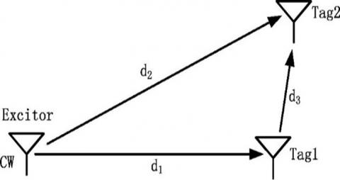
In the study [12], a passive backscattering tag-to-tag system was proposed where all tags can backscatter the CW signal and receive backscattered signals from other tags. Figure 1 shows a two-tag system in which the exciter broadcasts the CW signal so that both Tag 1 and Tag 2 can receive this signal; Tag 1 backscatters this signal and modulates it by varying its impedance between two states to convey the messages. In other words, the two tags can communicate with each other by backscattering and modulating the CW signal that is broadcasted by an external RF exciter. d1, d2 and d3 represent the distance between the Excitor and Tag 1, the distance between the Excitor and Tag 2, and the distance between the two tags, respectively. The objective is to model the received power for Tag 2 as a function of di where i=1, 2, 3.
Figure 1. The Tag-to-Tag communication system
Both ASK (Amplitude Shift Keying) and PSK (Phase Shift Keying) modulations were addressed [12]. In this paper, we focus on the case with ASK modulations where the tag alters the amplitude of the reflected signal in two states. The signal it receives is given by ϕ(t)=m(t)∙c(t) where m(t) is the binary sequence and c(t) is the carrier signal.
2.1 The total signal received by Tag 2 in ideal case
The total signal received by Tag 2 is a superposition of the backscattered signal from Tag 1 and the CW signal at Tag 2:
$s(t)=A_{E_2} \cos (2 \pi f t)+A_{T_1 T_2} \cos (2 \pi f t+\theta)$ (1)
where, $A_{E_2}$ is the amplitude of the received signal by Tag 2 from the Excitor, $A_{T_1 T_2}$ is the amplitude of the backscattered signal from Tag 1 to Tag 2, and θ is the phase difference between the CW signal and the Tag 1 backscattered signal at the Tag 2 antenna.
$\theta=\frac{2 \pi f\left(d_1+d_3-d_2\right)}{c}+\tilde{\theta}=\frac{2 \pi f \Delta d}{c}+\tilde{\theta}$, (2)
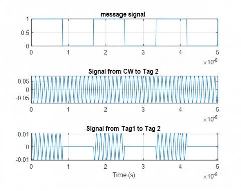
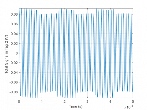
where, $\Delta d=d_1+d_3-d_2$ and $\tilde{\theta}$ is determined by the hardware and can be adjusted. Note that d2 can be found from $d_1, d_3$, and the angle using the cosine rule. Without loss of generality, we assume a straight triangle in the deployment. Figures 2 and 3 show the signals at $d_1=8 \mathrm{~m}$ and $d_3=0.5 \mathrm{~m}$ with a CW signal of frequency f=915MHz.
Figure 2. The signals at d1 = 8m and d3 = 0.5m
Figure 3. The total signal received at Tag 2 at d1 = 8m and d3 = 0.5m
From (1), we have $\begin{aligned} & s(t)=A_{E_2} \cos (2 \pi f t)+A_{T_1 T_2} \cos (2 \pi f t) \cos (\theta)- A_{T_1 T_2} \sin (2 \pi f t) \sin (\theta),\end{aligned}$ and therefore the amplitudes of s(t):
$\begin{array}{r}A_{T_2}=\sqrt{\left(A_{E_2}+A_{T_1 T_2} \cos \theta\right)^2+\left(A_{T_1 T_2} \sin \theta\right)^2} \\ =\sqrt{A_{E_2}^2+2 A_{E_2} A_{T_1 T_2} \cos \theta+A_{T_1 T_2}{ }^2}\end{array}$
The amplitudes of s(t) in two states for ASK (Note that in the ASK case, $\theta^{(1)}=\theta^{(2)}=\theta$.):
$A_{T_2}^{(1)}=\sqrt{A_{E_2}^2+2 A_{E_2} A_{T_1 T_2}^{(1)} \cos \theta^{(1)}+A_{T_1 T_2}^{(1)^2}}$, (3)
$A_{T_2}^{(2)}=\sqrt{A_{E_2}^2+2 A_{E_2} A_{T_1 T_2}^{(2)} \cos \theta^{(2)}+A_{T_1 T_2}^{(2)^2}}$, (4)
and the power of s(t) in two states:
$\begin{aligned} & P_{T_2}^{(1)}=P_{E_2}+2 \sqrt{P_{E_2} P_{T_1 T_2}^{(1)}} \cdot \cos \theta^{(1)}+P_{T_1 T_2}^{(1)} \\ & P_{T_2}^{(2)}=P_{E_2}+2 \sqrt{P_{E_2} P_{T_1 T_2}^{(2)}} \cdot \cos \theta^{(2)}+P_{T_1 T_2}^{(2)}\end{aligned}$ (5)
where, $P_{E_2}$ is the power received by Tag 2 from the Excitor, $P_{T_1 T_2}^{(1)}$ and $P_{T_1 T_2}^{(2)}$ are the power of the backscattered signal from Tag 1 to Tag 2 antenna in two states.
The power difference $\Delta P$:
$\begin{aligned} \Delta P=P_{T_2}^{(1)}-P_{T_2}^{(2)} & =2 \sqrt{P_{E_2}}\left(\sqrt{P_{T_1 T_2}^{(1)}} \cos \theta^{(1)}\right.\left.-\sqrt{P_{T_1 T_2}^{(2)}} \cos \theta^{(2)}\right) +\left(P_{T_1 T_2}^{(1)}-P_{T_1 T_2}^{(2)}\right)\end{aligned}$. (6)
The dB-power difference $\Delta P(d B)$ is defined to the difference between the $P_{T_2}^{(1)}(d B)$ and $P_{T_2}^{(2)}(d B)$ as shown in (7):
$\begin{gathered}\Delta P(d B)=P_{T_2}^{(1)}(d B)-P_{T_2}^{(2)}(d B) =10 \log _{10}\left(P_{E_2}+2 \sqrt{P_{E_2} P_{T_1 T_2}^{(1)}} \cdot \cos \theta^{(1)}+P_{T_1 T_2}^{(1)}\right) -10 \log _{10}\left(P_{E_2}+2 \sqrt{P_{E_2} P_{T_1 T_2}^{(2)}} \cdot \cos \theta^{(2)}+P_{T_1 T_2}^{(2)}\right)\end{gathered}$ (7)
Phase cancellation occurs at $A_{T_2}^{(1)}=A_{T_2}^{(2)}$ or $P_{T_2}^{(1)}=P_{T_2}^{(2)}$, where Tag 2 cannot detect and demodulate the signal sent from Tag 1. In order to mitigate the effect of the phase cancellation, a multiphase backscattering mechanism was proposed in the study [12] in which the tags uses different phases $\tilde{\theta}$ so that it creates diverse phase differences between the excitation signal and backscatter signal at Tag 2, resulting in different received power values and the higher one can be detected. Take a two-phase backscattering approach as an example. The tag will backscatter the same piece of information in two successive intervals with a phase difference implemented by different impedences of the tag antenna.
2.2 Log-normal propagation model
The expected received power is known as:
$\mathbb{E}\left[P_R\right]=P_T G_T G_R\left(\frac{\lambda}{4 \pi d}\right)^2$
by Friis equation [24]. The effect of shadowing is typically characterized by using the log-normal distribution and therefore the received power $P_R$ follows [25]:
$P_R(d B)=10 \log _{10} P_R \sim N\left(C_0-20 \log _{10} d, \sigma^2\right)$, (8)
where, $C_0=10 \log _{10} \frac{P_T G_T G_R \lambda^2}{(4 \pi)^2}$, d is the distance between the transmitter and the receiver, $\sigma$ is the standard deviation of the corresponding normal distribution. We have:
$f\left(P_R\right)=\frac{10 \log _{10} e}{P_R \sigma \sqrt{2 \pi}} \cdot e^{-\frac{\left(10 \log\,\, _{10} P_R-\left(C_0-20 \log\, _{10} d\right)\right)\,\,^2}{2 \sigma^2}}$
2.3 The power received by Tags from the Excitor: $P_{E_1}, P_{E_2}$
The power received by Tag 2 from the Excitor $P_{E_2}$ follows Eq. (8):
$P_{E_2}(d B) \triangleq 10 \log _{10} P_{E_2} \sim N\left(\mu_{E_2}, \sigma^2\right)$ (9)
That is, $P_{E_2}(d B)=\mu_{E_2}+X_\sigma$, where $\mu_{E_2}=C_0-20 \log _{10} d_2$ and $X_\sigma \sim N\left(0, \sigma^2\right)$. Therefore,
$\log _{10} d_2 \sim N\left(\frac{C_0-P_{E_2}(d B)}{20}, \frac{1}{20^2} \sigma^2\right)$ (10)
Similarly, the power received by Tag 1 from the Excitor $P_{E_1}$ follows:
$P_{E_1}(d B) \triangleq 10 \log _{10} P_{E_1} \sim N\left(\mu_{E_1}, \sigma^2\right)$ (11)
That is, $P_{E_1}(d B)=\mu_{E_1}+X_\sigma$, where $\mu_{E_1}=C_0-20 \log _{10} d_1$ and $X_\sigma \sim N\left(0, \sigma^2\right)$.
2.4 The power of the backscattered signal from Tag 1 to Tag 2: $P_{T_1 T_2}$
The expected power of the backscattered signal from Tag 1 to Tag 2: $\mathbb{E}\left[P_{T_1 T_2}\right]=\frac{k_1 P_{E 1} \cdot G_T G_R \lambda^2}{(4 \pi)^2 d_3^2}=k_1 \frac{P_T G_T G_R \lambda^2}{(4 \pi)^2 d_1^2} \cdot \frac{G_T G_R \lambda^2}{(4 \pi)^2 d_3^2}$. The power $P_{T_1 T_2}$ is assumed to follow the log-normal distribution: $P_{T_1 T_2}(d B)=\mu_{T_1 T_2}{ }^{\prime}+X_{\sigma_{T_1 T_2}}{ }^{\prime}$, where $X_{\sigma_{T_1 T_2}}^{\prime} \sim N\left(0, \sigma_{T_1 T_2}{ }^{\prime 2}\right)$ and $\mu_{T_1 T_2}{ }^{\prime}=10 \log _{10} k_1+10 \log _{10} P_{E_1}+C_0-20 \log _{10} d_3$. We obtained from the previous subsection that $10 \log _{10} P_{E_1}=\mu_{E_1}+X_\sigma=C_0-20 \log _{10} d_1+X_\sigma$.
Therefore,
$\begin{aligned} \mu_{T_1 T_2}{ }^{\prime}=10 \log _{10} & k_1+C_0-20 \log _{10} d_1+X_\sigma+C_0 \\ & -20 \log _{10} d_3 \Rightarrow P_{T_1 T_2}(d B)^{(1)} \\ & =10 \log _{10} k_1+C_0-20 \log _{10} d_1 \\ & +C_0-20 \log _{10} d_3+X_\sigma+X_{\sigma_{T_1 T_2}^{\prime}} \\ & \Rightarrow P_{T_1 T_2}(d B)^{(1)} \\ & \sim N\left(10 \log _{10} k_1+2 C_0\right. \\ & -20 \log _{10} d_1-20 \log _{10} d_3, \sigma^2 \\ & \left.+\sigma_{T_1 T_2}{ }^2\right)\end{aligned}$ (12)
Then we have:
$P_{T_1 T_2}^{(1)}(d B) \sim N\left(\mu_{T_1 T_2}^{(1)}, \sigma_{T_1 T_2}{ }^2\right)$ (13)
where, $\mu_{T_1 T_2}^{(1)}=10 \log _{10} k_1+2 C_0-20 \log _{10} d_1-20 \log _{10} d_3$ and $\sigma_{T_1 T_2}^2=\sigma^2+\sigma_{T_1 T_2}{ }^{\prime 2}$.
Similarly, we obtain the power in state 2:
$P_{T_1 T_2}^{(2)}(d B) \sim N\left(\mu_{T_1 T_2}^{(2)}, \sigma_{T_1 T_2}{ }^2\right)$ (14)
where, $\mu_{T_1 T_2}^{(2)}=10 \log _{10} k_2+2 C_0-20 \log _{10} d_1-20 \log _{10} d_3$ and $\sigma_{T_1 T_2}^2=\sigma^2+\sigma_{T_1 T_2}{ }^{\prime 2}$.
3.1 The likelihood function
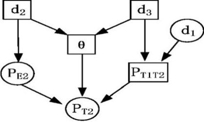
Figure 4 shows the relationship among all the variables where the squares represent the observable variable and the circles represent the hidden variables. Let Let $y \triangleq \Delta P(d B)$. Because it is complicated to find an analytical solution for the modeling of the likelihood function $f\left(y \mid d_3\right)$, this section aims at deriving an analytically tractable observation model for the later use in localization and tracking problems.
Suppose the modified method introduced in section 2 is applied using N different phases with equal interval within 2π. Let γ=2cosθ, where θ is the phase difference in Eq. (2). Several assumptions are made as follows in this section.
Assumption 1: On-off switching case (OOK).
Assumption 2: We applied 4 different phases with interval $\frac{\pi}{2}$ for the modified method.
Assumption 3: γ is a constant.
Lemma 1 Under Assumption 1, $P_{T_2}^{(2)}=P_{E_2}$.
Proof: In the case of OOK, $P_{T_1 T_2}^{(2)}=0$ in state 2 and hence $P_{T_2}^{(2)}=P_{E_2}$ from Eq. (5).
Lemma 2 Under Assumption 2, $\sqrt{2} \leq \max \{\gamma\} \leq 2$.
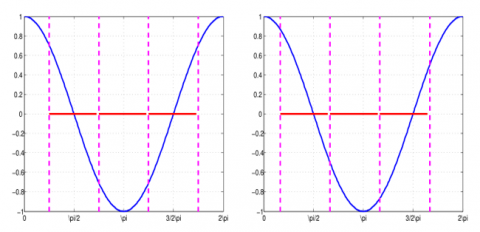
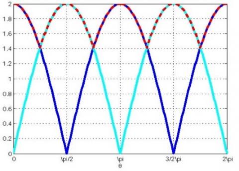
Proof: Two examples are shown in Figure 5 in the case of four phase differences $\theta \in\left\{\theta_0, \theta_0+\pi / 2, \theta_0+\pi, \theta_0+3 \pi / 2\right\}$. Let $\begin{aligned} & \gamma^{\prime}=\max \{2 \cos \theta\}=\max \left\{2 \cos \theta_0, 2 \cos \left(\theta_0+\pi /\right.\right. \left.2), 2 \cos \left(\theta_0+\pi\right), 2 \cos \left(\theta_0+3 \pi / 2\right)\right\}= \max \left\{2 \cos \theta_0,-2 \sin \theta_0,-2 \cos \theta_0, 2 \sin \theta_0\right\}= \max \left\{2\left|\cos \theta_0\right|, 2\left|\sin \theta_0\right|\right\}\end{aligned}$ as shown in Figure 6. It can be shown that the minimum value of $\gamma^{\prime}$ is $\frac{\sqrt{2}}{2}$ when $\theta=\pm \frac{\pi}{4}+2 k \pi$ and the maximum value is 1 when θ=2kπ or θ=π/2+2kπ.
Lemma 3 When N→+∞, γ achieves its maximum value and max{γ}=2.
Proof: $\tilde{\theta}=\left\{\theta_0, \theta_0+\Delta \theta_1, \theta_0+\Delta \theta_2, \cdots, \theta_0+\Delta \theta_N\right\}$. It is obvious that when N→+∞, $\tilde{\theta}$ is guaranteed to reach 2π and therefore $\max \{\gamma\}=2 \max \{\cos \tilde{\theta}\}=2 \cos (2 \pi)=2$.
Lemma 4 When N→+∞, the maximum power difference is obtained.
Proof: With Assumption 2 and Lemma 2, $N \rightarrow+\infty \Rightarrow \max \{\gamma\}$. From Eq. (5), $\max \{\gamma\} \Rightarrow \max \left\{P_{T_2}^{(1)}\right\}$. With Assumption 1 and Eq. (6) we have $\Delta P=P_{T_2}^{(1)}-P_{E_2}$ and hence $\max \left\{P_{T_2}^{(1)}\right\} \Rightarrow \max \{\Delta P\}$. Therefore, the maximum power difference $\Delta P$ is obtained. Recall that Phase cancellation was defined to be when $\Delta P=0$ and it occurs when the tag is unable to distinguish between the signals under the two states. Lemma 4 provides a theoretical basis for the multiphase backcattering approach to address the Phase cancellation problem because the larger the power difference $\Delta P$, the easier for the tag to distiguish between the two states.
From Eq. (5), we have $\begin{aligned} P_{T_2}^{(1)} & =P_{E_2}+\gamma \sqrt{P_{E_2} P_{T_1 T_2}}+P_{T_1 T_2}=P_{E_2}\left(1+\gamma \sqrt{\frac{P_{T_1 T_2}}{P_{E_2}}}+\right. \left.\frac{P_{T_1 T_2}}{P_{E_2}}\right) & =P_{E_2}\left(1+\gamma P_x+P_x^2\right)\end{aligned}$,
where, $P_x \triangleq \sqrt{\frac{P_{T_1 T_2}}{P_{E_2}}}$ and $P_x \ll 1$, then:
$\begin{gathered}10 \log _{10} P_{T_2}^{(1)}=10 \log _{10} P_{E_2}+10 \log _{10}\left(1+\gamma P_x\right. \left.+P_x^2\right)\end{gathered}$, (15)
where, $\log _{10}\left(1+\gamma P_x+P_x^2\right) \approx \log _{10}\left(1+\gamma P_x\right) \approx \gamma P_x / \ln 10$.
Therefore $P_{T_2}(d B)^{(1)}=P_{E_2}(d B)+10 \gamma P_x / \ln 10$. From Eq. (7), $\begin{aligned} & \Delta P(d B)=P_{T_2}(d B)^{(1)}-P_{T_2}(d B)^{(2)}=P_{T_2}(d B)^{(1)}- P_{E_2}(d B)\end{aligned}$ due to Lemma 1. We obtain that $\Delta P(d B)=10 \gamma P_x / \ln 10$.
Let $\Psi \triangleq 10 \log _{10} \Delta P(d B)$ and we have,
$\Psi=10 \log _{10}\left(\frac{10 \gamma P_x}{\ln 10}\right)=10 \log _{10}\left(\frac{10 \gamma}{\ln 10}\right)+P_x(d B)$ (16)
where, $P_x(d B)=10 \log _{10} \sqrt{\frac{P_{T_1 T_2}}{P_{E_2}}}=\frac{P_{T_1 T_2}(d B)-P_{E_2}(d B)}{2}$.
We already have $P_{T_1 T_2}(d B) \sim N\left(\mu_{T_1 T_2}, \sigma_{T_1 T_2}{ }^2\right)$ and $P_{E_2}(d B) \sim N\left(\mu_{E_2}, \sigma^2\right)$.
$\begin{aligned} P_x(d B) & =\frac{\left(\mu_{T_1 T_2}+X_{\sigma_{T_1 T_2}}\right)-\left(\mu_{E_2}+X_\sigma\right)}{2} =\frac{\mu_{T_1 T_2}-\mu_{E_2}+X_{\sigma_{T_1 T_2}}-X_\sigma}{2}\end{aligned}$
$X_{\sigma_{T_1 T_2}}$ and $X_\sigma$ are assumed to be independent. Given $d_i$, where i=1,2,3, We have:
$\Psi \sim N\left(\mu_3, \sigma_3^2\right)$, (17)
where, $\begin{aligned} & \mu_3=10 \log _{10}(10 y / \ln 10)+\frac{\mu_{T_1 T_2}-\mu_{E_2}}{2} =10 \log _{10}\left(\frac{10}{\ln 10}\right)+10 \log _{10} \gamma+\frac{\left(10 \log _{10} k_1+2 C_0-20 \log _{10} d_1-20 \log _{10} d_3\right)-\left(C_0-20 \log _{10} d_2\right)}{2} =10 \log _{10}(10 / \ln 10)+10 \log _{10} \gamma+\frac{10 \log _{10} k_1+C_0-20 \log _{10} d_1-20 \log _{10} d_3+20 \log _{10} d_2}{2} =c_0+10 \log _{10} \gamma+\frac{10 \log _{10} k_1+C_0-20 \log _{10} d_1-20 \log _{10} d_3+20 \log _{10} d_2}{2}\end{aligned}$ and $\sigma_3=\frac{\sigma_{T_1 T_2}^2+\sigma^2}{4}$, where q, $c_0=10 \log _{10}(10 / \ln 10)$ is a constant.
Therefore, the likelihood function is:
$f\left(y \mid d_i\right)=\frac{1og \,_{10} e}{y \sqrt{2 \pi} \sigma_3} \cdot e^{-\frac{\left(y-\frac{\mu\,_3}{10}\right)^2}{2\left(\frac{\sigma_3}{10}\right)^2}}$
Figure 4. The relationship
Figure 5. Two examples of four phases with a $\frac{\pi}{2}$ interval in one period, the magenta dashed lines represent the values cos(θ) of the four phases
Figure 6. The blue and the cyan lines show the curves of $2|\cos (\theta)|$ and $2|\sin (\theta)|$, and $2|\sin (\theta)|$, respectively, the dashed red line shows the curve of $\gamma=\max \{2|\cos (\theta)|, 2|\sin (\theta)|\}$
3.2 Simulation and analysis
3.2.1 With γ known
In this subsection we simulated the case when γ is assumed to be fixed and known both in the cases of γ=2 and $\gamma=\max \left\{2 \cos \theta_i, i=1,2,3,4\right\}$, where $\theta_i$ is i-th phase in a 4-phase backscattering mechanism. We denote this model as the Fixed-γ Model (FIM).
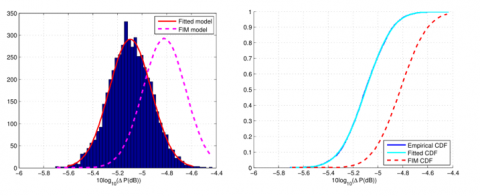
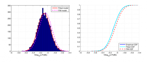
The simulation results are shown with $d_3=1.5 \mathrm{~m}$ in Figure 7 assuming γ=2. The means from numerical data and from our proposed FIM model are -5.0971 and -4.8205 respectively. The variance from both cases are 0.0292 and 0.0300. One reason of the deviation of the FIM modeling is due to the assumption of γ=2. By Lemma 3, γ=2 when N→∞, however, we only applied four different $\tilde{\theta}$. The mismatch occurs between the assumption γ=2 and the fact N=4. Figure 8 shows the results of the FIM model with γ being assumed to be exactly known. The mean and the variance are -5.0573 and 0.0300, respectively.
Figure 7. The pdf and cdf of ψ assuming γ=2
Figure 8. The pdf and cdf of ψ assuming $\gamma=\max \left\{2 \cos \left(\theta_i\right), i=1,2,3,4\right\}$ can be obtained
3.2.2 With γ unknown
In the previous subsection, $\gamma$ is assumed to fixed and known. Now we release this assumption and propose a random variable γ=2cosθ with θ∼Unif(0,π/4). From Eq. (17), $\Psi \sim N\left(\mu_3, \sigma_3^2\right)$, $\mu_3=c_0+10 \log _{10} \gamma+\mu_0$ where $\mu_0=\frac{\mu_{T_1 T_2}-\mu_{E_2}}{2}$, where $\mu_3=c_0+10 \log _{10} \gamma+\mu_0$, our objective is to find the distribution of $z=10 \log _{10} \gamma$.
$\theta \sim \operatorname{Unif}(0, \pi / 4), \quad \gamma=2 \cos \theta$
$f_{\Theta}(\theta)= \begin{cases}\frac{4}{\pi}, & 0 \leq \theta \leq \frac{\pi}{4} \\ 0, & 0 . w .\end{cases}$
$\begin{aligned} \theta=\arccos \frac{\gamma}{2}, & g^{\prime}(\theta)=-2 \sin \theta=-\sqrt{4-\gamma^2} \Rightarrow f_{\Gamma}(\gamma) \\ = & \frac{f_{\Theta}(\theta)}{\left|g^{\prime}(\theta)\right|}=\frac{4}{\pi \sqrt{4-\gamma^2}} \text { when } \sqrt{2} \leq \gamma \leq 2 \\ \Rightarrow & f_{\Gamma}(\gamma)= \begin{cases}\frac{4}{\pi \sqrt{4-\gamma^2}}, & \sqrt{2} \leq \gamma \leq 2 \\ 0, & \text { o.w. }\end{cases} \end{aligned}$
Let $z=10 \log _{10} \gamma \Rightarrow \gamma=10^{\frac{2}{10}}, g^{\prime}(\gamma)=\frac{10}{\gamma \ln 10}=\frac{10}{10^{\frac{z}{10}} \ln 10}$,
$\Rightarrow f_Z(z)= \begin{cases}\frac{4(\ln 10) 10^{\frac{z}{10}}}{} \\ \frac{\pi \sqrt{4-10^{\frac{z}{5}}}}{10}, & 5 \log _{10} 2 \leq \gamma \leq 20 \log _{10} 2 \\ 0, & \text { o.w. }\end{cases}$$\begin{aligned} & \Rightarrow f_Z(z) \\ & = \begin{cases}\frac{2(\ln 10)}{5 \pi \sqrt{4 \cdot 10^{-\frac{z}{10}}-1}}, & 5 \log _{10} 2 \leq \gamma \leq 20 \log _{10} 2 \\ 0, & \text { o.w. }\end{cases} \end{aligned}$ (18)
We have:
$\begin{aligned} f\left(\Psi \mid z, d_i\right) & =\frac{1}{\sqrt{2 \pi} \sigma_3} \cdot e^{-\frac{\left(\Psi-\left(c\,_0+z+\mu_0\right)\right)\,\,^2}{2 \sigma_3^2}} \\ f\left(\Psi \mid d_i\right) & =\int_Z f\left(\Psi \mid z, d_i\right) f_Z(z) d z\end{aligned}$ (19)
$\begin{aligned} & =\int_{5 \log _{10} 2}^{20 \log _{10} 2} \frac{1}{\sqrt{2 \pi} \sigma_3} \cdot e^{-\frac{\left(\Psi-\left(c_0+z+\mu_0\right)\right)^2}{2 \sigma_3^2}} \frac{2(\ln 10)}{5 \pi \sqrt{4 \cdot 10^{-\frac{z}{10}}-1}} d z =\int_{5 \log _{10} 2}^{20 \log _{10} 2} \frac{2(\ln 10)}{5 \sqrt{2 \pi^3} \sigma_3} \cdot e^{-\frac{\left(\Psi-\left(c_0+z+\mu_0\right)\right)\,\,^2}{2 \sigma_3^2}} . \frac{1}{\sqrt{4 \cdot 10^{-\frac{z}{10}}-1}} d z \end{aligned}$ (20)
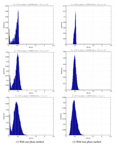
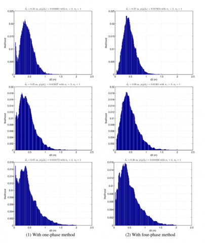
Figures 9 and 10 show the likelihood function $f\left(y \mid d_3\right)$ with original one-phase method and the modified four-phase method. Table 1 shows the likelihood values when $d_3=0.5 \mathrm{~m}$ and the estimation results of $d_3$ using maximum likelihood method [26]. We can see that the modified method with four phases performs much better than the original method especially in the cases of large variance σ. For example, with σ=[4, 1], the estimated distance value of $d_3$ (when $d_3$ was set to be 0.5 m) using one-phase method is 0.05 m and that using four-phase method is 0.36 m.
Figure 9. The likelihood function of the log-power difference $\Delta \mathrm{P}(\mathrm{dB})$ with different low noise variances with the two methods
Figure 10. The likelihood function of the log-power difference ΔP(dB) with different high noise variances with the two methods
Table 1. The estimation performance where $\tilde{\mathrm{d}}_3$ is the estimated distance between Tag1 and Tag2
|
Variable |
Method |
σ |
|||||
|
[0.1,0.1] |
[0.5,0.5] |
[1, 1] |
[2, 1] |
[3, 1] |
[4, 1] |
||
|
$\widetilde{d_3}$ |
One-phase |
0.54 |
0.49 |
0.41 |
0.37 |
0.25 |
0.05 |
|
Four-phase |
0.53 |
0.48 |
0.47 |
0.41 |
0.36 |
0.36 |
|
This study shows that the log-power difference can be utilized as observations for the localization and tracking problems. We also shows the numerical results of the likelihood function of the log-power difference, and estimate the distance between the two tags using maximum likehood estimation based on our proposed observation model. The results demonstrate the advantages of the modified method with multiphase backscattering where it shows a significantly improved estimation accuracy with more phases. We further extend the analysis to an infinite number of phases in spite of the hardware limitation. The presented work is a first basis to the localization and tracking problems in passive tag-to-tag communication systems where a realistic observation model is essential. Our future work includes to generalize the model for an arbitrary number of phases, extend it to the case with other modulations, and to employ this model to address a practical localization and tracking problem.
This work was partly supported by PSC-CUNY grant #63160-00 51, funded by the Professional Staff Congress of the City University of New York.
|
$A_{E_2}$ |
the amplitude of the received signal by Tag 2 from the Excitor |
|
$A_{T_2}^{(i)}$ |
the amplitude of the total received signal by Tag 2 in state $i(i \in\{1,2\})$ |
|
$A_{T_1 T_2}^{(i)}$ |
the amplitude of the backscattered signal from Tag 1 to Tag 2 in state i |
|
$d_1$ |
distance between the Excitor and Tag 1 |
|
$d_2$ |
distance between the Excitor and Tag 2 |
|
$d_3$ |
distance between Tag 1 and Tag 2 |
|
$k_1$ |
the K factor (The K factor is the ratio of the backscattered power and the maximum absorbed power delivered to the matched load) in state 1 |
|
$k_2$ |
the K factor in state 2 |
|
$P_{E_1}$ |
the power received by Tag 1 from the Excitor |
|
$P_{E_2}$ |
the power received by Tag 2 from the Excitor |
|
$P_{T_2}^{(i)}$ |
the total power received by Tag 2 in state i |
|
$P_{T_1 T_2}^{(i)}$ |
the power of the backscattered signal from Tag 1 to Tag 2 in state i |
|
$\Delta P$ |
the received power difference between the two states |
|
$\theta^{(i)}$ |
the phase difference in state i |
|
$\tilde{\theta}$ |
the adjustable phase |
|
λ |
the wavelength |
[1] Finkenzeller, K. (2010). RFID handbook. Wiley, New York.
[2] Steiner Kopetz, H. (2022). Internet of Things. In: Real-Time Systems, Springer, Cham.
[3] Abubakar, S., Jun, O., Kamran, A., Muhammad, A.I., Qammer, H.A. (2021) Passive UHF RFID tag antennas-based sensing for internet of things paradigm. Backscattering and RF Sensing for Future Wireless Communication, pp. 133-155. http://dx.doi.org/10.1002/9781119695721.ch7
[4] Shan, H.Y., Peterson III, J., Hathorn, S., Mohammadi, S. (2018) The RFID connection: RFID technology for sensing and the internet of things. IEEE Microwave Magazine, 19(7): 63-79. http://dx.doi.org/10.1109/MMM.2018.2863439
[5] Liu, V., Parks, A., Talla, V., Gollakota, S., Wetherall, D., Smith, J.R. (2013). Ambient backscatter: Wireless communication out of thin air. In Proceedings of the ACM SIGCOMM, 43(4): 39-50. https://doi.org/10.1145/2534169.2486015
[6] Sample, A.P., Yeager, D.J., Powledge, P.S., Mamishev, A.V., Smith, J.R. (2008). Design of an RFID-based battery-free programmable sensing platform. IEEE Transactions on Instrumentation and Measurement, 57(11): 2608-2615. http://dx.doi.org/10.1109/TIM.2008.925019
[7] Zhang, H., Gummeson, J., Ransford, B., Fu, K. (2011). Moo: A batteryless computational RFID and sensing platform. University of Massachusetts Computer Science Technical Report UM-CS-2011-020. https://web.cs.umass.edu/publication/docs/2011/UM-CS-2011-020.pdf.
[8] Joshua, F.E., Matthew, S.R. (2015). Every smart phone is a backscatter reader: Modulated backscatter compatibility with bluetooth 4.0 low energy (BLE) devices. In 2015 IEEE International Conference on RFID, pp. 78-85. http://dx.doi.org/10.1109/RFID.2015.7113076
[9] Zhang, P.Y., Bharadia, D., Joshi, K., Katti, S. (2016). Hitchhike: Practical backscatter using commodity Wi-Fi. In Proceedings of the 14th ACM Conference on Embedded Network Sensor Systems CD-ROM, pp. 259-271. http://dx.doi.org/10.1145/2994551.2994565
[10] Zhang, P.Y., Josephson, C., Bharadia, D., Katti, S. (2017) Freerider: Backscatter communication using commodity radios. In Proceedings of the 13th International Conference on emerging Networking Experiments and Technologies, pp. 389-401. http://dx.doi.org/10.1145/3143361.3143374
[11] Martinez, R., Nikitin, P.V., Ramamurthy, S., Rao, K.V.S. (2012). Passive tag-to-tag communication. In IEEE International Conference on RFID (RFID), pp. 177-184. https://doi.org/10.1109/RFID.2012.6193048
[12] Shen, Z., Athalye, A, Petar, M.D. (2016) Phase cancellation in backscatter-based tag-to-tag communication systems. IEEE Internet of Things Journal, 3(6): 959-970. http://dx.doi.org/10.1109/JIOT.2016.2533398
[13] Ryoo, J., Jian, J.H., Athalye, A., Samir, R.D., Milutin, S. (2018) Design and evaluation of BTTN: A backscattering tag-to-tag network. IEEE Internet of Things Journal, 5(4): 2844-2855. http://dx.doi.org/10.1109/JIOT.2018.2840144
[14] Majid, A.Y., Jansen, M., Delgado, G.O., Yildirim, K.S., Pawellzak, P. (2019). Multi-hop backscatter tag-to-tag networks. In IEEE INFOCOM 2019-IEEE Conference on Computer Communications, pp. 721-729. http://dx.doi.org/10.1109/INFOCOM.2019.8737551
[15] Lassouaoui, T., Hutu, F.D., Duroc, Y., Villemaud, G. (2022). Performance evaluation of passive tag to tag communications. IEEE Access, 10: 18832-18842. http://dx.doi.org/10.1109/ACCESS.2022.3149626
[16] Li, G., Monica, F.B., Athalye, A., Petar, M.D. (2015). Real-time self-tracking in the internet of things. In 2015 IEEE International Conference on Acoustics, Speech and Signal Processing (ICASSP), pp. 5510-5514. http://dx.doi.org/10.1109/ICASSP.2015.7179025
[17] Ahmad, A., Huang, Y.F., Sha, X., Athalye, A., Stanacevic, M., Samir, R.D., Petar, M.D. (2020). On measuring doppler shifts between tags in a backscattering tag-to-tag network with applications in tracking. In ICASSP 2020-2020 IEEE International Conference on Acoustics, Speech and Signal Processing (ICASSP), pp. 9055-9059. http://dx.doi.org/10.1109/ICASSP40776.2020.9053291
[18] Vorst, P., Zell, A. (2008). Semi-autonomous learning of an RFID sensor model for mobile robot self-localization. In European Robotics Symposium. Springer, pp. 273-282. http://dx.doi.org/10.1007/978-3-540-78317-6_28
[19] Joho, D., Plagemann, C., Burgard, W. (2009). Modeling RFID signal strength and tag detection for localization and mapping. In Proceedings of the IEEE International Conference on Robotics and Automation (ICRA), pp. 3160-3165. http://dx.doi.org/10.1109/ROBOT.2009.5152372
[20] Milella, A., Cicirelli, G., Distante, A. (2008). RFID-assisted mobile robot system for mapping and surveillance of indoor environments. Industrial Robot: An International Journal, 35(2): 143-152. http://dx.doi.org/10.1108/01439910810854638
[21] Geng, L., Bugallo, M.F., Athalye, A., Djuri´c, P.M. (2014). Indoor tracking with RFID systems. IEEE Journal of Selected Topics in Signal Processing, 8(1): 96-105. http://dx.doi.org/10.1109/JSTSP.2013.2286972
[22] Doucet, A., Freitas, N., Gordon, N. (2001). Sequential monte carlo methods in practice. Springer, New York. http://dx.doi.org/10.1007/978-1-4757-3437-9
[23] Risti´c, B., Arulampalam, S., Gordon, N. (2004). Beyond the kalman filter: Particle filters for tracking applications. Artech House Publishers. http://www.fusion2004.foi.se/papers/IF04-0502.pdf.
[24] Dobkin, D. (2007). The RF in RFID: Passive UHF RFID in practice.
[25] Sarkar, T., Ji, Z., Kim, K., Medouri, A., Salazar-Palma, M. (2003). A survey of various propagation models for mobile communication. IEEE Antennas and Propagation Magazine, 45(3): 51-82. http://dx.doi.org/10.1109/MAP.2003.1232163
[26] Rossi, R.J. (2018). Mathematical Statistics: An Introduction to Likelihood Based Inference. New York: John Wiley & Sons. http://dx.doi.org/10.1002/9781118771075