Agung Prayitno* | Veronica Indrawati | Itthisek Nilkhamhang
© 2022 IIETA. This article is published by IIETA and is licensed under the CC BY 4.0 license (http://creativecommons.org/licenses/by/4.0/).
OPEN ACCESS
Many distributed controllers for vehicle platoon are designed based on homogeneous assumption and full state information. In reality, vehicle platoon may consist of heterogeneous vehicles and may have limited information due to sensor constraints. Therefore, this paper proposes a distributed model reference adaptive control based on cooperative observer for a heterogeneous vehicle platoon with limited output information and subjected to uncertain dynamics. Cooperative observer provides a full state estimation of the system. Each follower has a reference model that is designed based on its nominal model and cooperative state variable feedback. Main control system is composed of (i) nominal control that utilized the cooperative state estimation tracking error and (ii) adaptive term that adopted an optimal control modification as an adaptation law. The tracking error of followers to the reference model is shown uniformly bounded and the stability of the platoon is guaranteed through detailed analysis. Performance of the proposed controller is verified by using numerical simulation. To show the advantage of the proposed control, simulation results are compared to the standard distributed model reference adaptive control that is applied for heterogeneous vehicle platoon. It is shown that the proposed control eliminated the high frequency oscillation in the control input.
cooperative observer design, distributed model reference adaptive control, heterogeneous vehicle platoon, optimal control modification
Research on vehicle and transportation technology is progressing rapidly, including electric vehicles [1], autonomous vehicles [2, 3], connected vehicles [2], traffic management [4] and the possibility of collaboration between unmanned ground vehicles and unmanned aerial vehicles [5]. As we know that the future of transportation is predicted to be connected and automated which allows information to be exchanged between vehicles, pedestrians and infrastructures in the intelligent transportation system (ITS) scheme. With this comprehensive information, various features of cooperative control between vehicles can be embedded in the vehicle for various purposes such as increasing safety, obtaining information about emergency situations, receiving weather reports, creating eco-friendly driving modes and enhancing vehicle mobility. This paper focuses on the aspect of enhancing vehicle mobility with a feature known as a vehicle platoon. Vehicle platoon is a group of vehicles, consisting of 1 leader and N-followers connected via a network of sensors or wireless communication technology, forms a convoy by synchronizing the followers’ velocity and acceleration to the leader's state while keeping the desired inter-vehicle distance. Vehicle platoon offers many advantages such as to improve safety and comfort driving, reduce congestion, maximize road capacity, save fuel and reduce air pollution [2]. Therefore, the development of vehicle platoon is a promising breakthrough in the future transportation technology.
Vehicle platoon structure, in multi-agent system (MAS) perspective, is composed of vehicle longitudinal dynamics, information flow topology, spacing policy and distributed controller [6]. In linearized third-order vehicle model [7], vehicle dynamics is depended on its inertial time lag where the value is different from one type vehicle to the others. Vehicle platoon that consists of vehicles with identical inertial time lags is called as a homogeneous vehicle platoon [8]. While, vehicles involved in a heterogeneous vehicle platoon have various inertial time lags [9]. Vehicles exchange information to the other vehicles via inter-vehicle communication technology according to the topology that is used which can either be a directed [10] or undirected topology [11]. There are some common topologies used by researchers for vehicle platoon applications. In directed topologies, four common topologies are used, namely predecessor following (PF) [12], two-predecessor following (TPF) [13], predecessor following leader (PFL) [14], two-predecessor following leader (TPFL) [8]. While, bidirectional (BD) [15] and bidirectional leader (BDL) [8] are common for undirected topologies. To achieve synchronization, a distributed controller is applied to each follower based on specific spacing policy which can either be constant spacing policy (CSP) [16] or constant time heading (CTH) [12].
Since the complexity of real vehicle dynamics, uncertain dynamics is inevitable. The uncertain dynamics can be a result of modeling error [17] or can also be a result of operating condition such as road and vehicle conditions, and environmental factors [9]. Therefore, the uncertain dynamics should be considered in the distributed controller design. A nominal control is a controller that designed based on a nominal model without considering its uncertain dynamics. This controller may decline in performance when the actual vehicle dynamics deviates significantly from its nominal model. In extreme situation, instability of the system may not be avoided [9]. Many literatures have been proposed to handle this issue either for general leader-follower problem or vehicle platoon applications. In order to solve the unknown matched uncertainty and disturbance for general leader-follower MAS, Peng et al. [18] designed a distributed model reference adaptive control. However, leader state is used as a reference model, which will be difficult for followers with no directly communication to the leader. For specific vehicle platoon with CTH and predecessor-following topology, an augmented model reference adaptive control approach was developed by Harfouch et al. [12], while Song et al. [19] designed a set of robust delay feedback controllers. Recently, distributed model reference adaptive control (DMRAC) which has reference model based on its follower’s nominal model was proposed by Prayitno et al. [20] for vehicle platoons with CSP and can be applied to various directed and undirected topologies. However, researchers [12, 18, 20] assumed a homogenous system where all platoon vehicles share an identical nominal model.
Homogeneous assumption limits the practicality since in the road, vehicles have different types and manucfaturers [9, 21]. Therefore, a vehicle platoon may consist of passenger cars, buses, vans, trucks and container trucks with variation of brands. This group of vehicles can be categorized as a heterogeneous vehicle platoon. Heavy duty vehicles typically have bigger inertial time lag when compared to passenger vehicles [10]. Since heterogenous vehicles have variation in inertial time lag, each individual vehicle may not perform optimally when the controller is designed based on an identical nominal model that has significant differences from the actual model. Zheng et al. [10] provided controller synthesis and analysis of cooperative control of heterogeneous vehicle platoon for directed acyclic interactions without considering the uncertain dynamics. Applying heterogeneous distributed controller for heterogeneous vehicle platoon subjected to uncertain dynamics is quite challenging. Recently, DMRAC is applied for synchronization of heterogeneous vehicle platoon subjected to uncertain dynamics [22]. However, it still has a problem of high frequency oscillation in the control input. The problem usually happens when fast adaptation is selected [22, 23], which may cause vehicle jerk and energy inefficiency. It is known that large jerk causing less comfort in the driving [24]. However, in certain condition, fast adaptation is required to improve the tracking performance especially when significant uncertainty occurred in the vehicle due to structural damage in the vehicle [25].
Many existing cooperative controllers for general leader-follower MAS or vehicle platoon are designed based on the assumption that full-state information are available or can be measured [10, 18, 20]. This assumption may make difficulty when full-state information is not available in each follower vehicle. In order to solve this problem, cooperative observer was proposed [26, 27] which utilized neighborhood output estimation error to provide follower’s full-state estimation. By utilizing the cooperative state estimation tracking error, a synchronization control to the leader is designed. However, work [26, 27] is designed based on nominal model and applied for homogeneous system.
Consequently, this paper proposes DMRAC based on cooperative observer to achieve synchronization of heterogeneous vehicle platoons subjected to uncertain dynamics. Reference model is designed based on heterogeneous cooperative state variable feedback control (CSVFB). While, main control is composed of a nominal control signal and an adaptive term. In order to solve the problem of high frequency oscillation control input, an optimal control modification (OCM) [28] is adopted as an adaptation law which extended the application for cooperative tracking problem. The main contributions of this paper are:
Compared to the references [18, 20, 22], the proposed control is designed based on cooperative observer which can be applied for vehicle with limited output information. Compared to the references [10, 26], the proposed control is extended the results to include the uncertain dynamics.
Provides the stability analysis of DMARC with OCM which derived based on cooperative tracking problem. DMRAC with OCM eliminates high frequency oscillation in the control input which usually occurred in the standard DMRAC [22] with high adaptation rate.
The rest of the paper presents the problem formulation, details of the proposed controller and main result which will be followed by stability proof. Finally, the performance of the proposed controller is validated through numerical simulations.
Information flow between followers involved in the platoon can be represented by a graph. Denote a graph as $\mathcal{G}(\mathcal{V}, \mathcal{E}, \mathcal{A})$, where $\mathcal{V}=\left\{v_1, v_2, \ldots, v_N\right\}$ is a set of nodes (followers), $\mathcal{E} \subseteq$ $\mathcal{V} \times \mathcal{V}$ is a set of links between the followers and $\mathcal{A}=\left[a_{i j}\right] \in$ $\mathbb{R}^{N \times N}$ is an adjacency matrix to represent the information exchange between followers. aij=1 if and only if follower i can receive information from follower j, otherwise aij=0. The in-degree matrix is defined as $D=\operatorname{diag}\left\{d_{11}, d_{22}, \ldots, d_{N N}\right\}$, where $d_{i i}=\sum_{j=1}^N a_{i j}$. The Laplacian matrix is represented by $L=\left[\ell_{i j}\right]=D-\mathcal{A} \in$ $\mathbb{R}^{N \times N}$ where $\ell_{i i}=d_{i i}$, and the other elements, $\ell_{i j}=-a_{i j}$. A pinning gain matrix is defined as $G=\operatorname{diag}\left\{g_{11}, g_{22}, \ldots, g_{N N}\right\}$, where $g_{i i}=1$ means that follower $i$ receives direct information from the leader, otherwise $g_{i i}=0$. Let $\tilde{\mathcal{G}}(\tilde{\mathcal{V}}, \tilde{\mathcal{E}})$ be defined such that $\tilde{\mathcal{V}}=\left\{v_0, v_1, v_2, \ldots, v_N\right\}$ and $\tilde{\mathcal{E}} \subseteq \tilde{\mathcal{V}} \times \tilde{\mathcal{V}}$ are directed from one node to another node. A topology of vehicle platoon contains a spanning tree if from the leader (as a root node) all followers can be reached by following link arrows.
Assumption 1: $\tilde{\mathcal{G}}$ of vehicle platoon is directed and has at least one spanning tree with the lead vehicle as a root node [29].
Consider a vehicle platoon, where the followers’ dynamics can be described as,
$\dot{x}_i=A_i x_i+B_i \Omega_i u_i+B_i \eta_i\left(x_i\right)$ (1)
$y_i=C_i x_i$ (2)
where, $x_i=\left[\begin{array}{lll}p_i+i \cdot d_r & v_i & a_i\end{array}\right]^T$ is the ith follower’s state and $y_i \in \mathbb{R}^p$ is the i th follower’s output. $u_i \in \mathbb{R}^m, \Omega_i, \eta_i\left(x_i\right)$ are the control input, control effectiveness, unknown matched uncertainty of the ith follower respectively. The uncertainty is parameterized as $\eta_i\left(x_i\right)=W_i^T \sigma_i\left(x_i\right)$ where $W_i \in \mathbb{R}^{s \times m}$ is an unknown constant weighting matrix and $\sigma_i\left(x_i\right): \mathbb{R}^n \rightarrow \mathbb{R}^s$ is a known basis vector function [17].
The leader has a zero input, which can be described as,
$\dot{x}_0=A_0 x_0$ (3)
$y_0=C_0 x_0$ (4)
where, $x_0=\left[\begin{array}{lll}p_0 & v_0 & a_0\end{array}\right]^T$ is the leader’s state and $y_0 \in \mathbb{R}^p$ is the leader’s output. Here, $p_i, v_i$ and $a_i$ for all $i \in\{0,1, \ldots, N\}$ are the position, velocity and acceleration of the ith vehicle respectively. While $A_i, B_i$, and $C_i$ are the system matrix, control matrix, and output matrix of the ith vehicle respectively. By defining $\tau_i$ as the inertial time lag of the powertrain, $A_i$ and $B_i$ are represented by
$A_i=\left[\begin{array}{ccc}0 & 1 & 0 \\ 0 & 0 & 1 \\ 0 & 0 & -\frac{1}{\tau_i}\end{array}\right], B_i=\left[\begin{array}{l}0 \\ 0 \\ \frac{1}{\tau_i}\end{array}\right], i \in\{0,1, ., N\}$ (5)
It is assumed that full state information is not available in each follower. Therefore, a dynamical output regulator in each follower can be designed based on state observers which utilize the available output measurements. Observer provides a full state estimation of the follower, which will be utilized for nominal controller design. Denote the estimation of $x_i$ as $\hat{x}_i$, while the estimation of $y_i$ as $\hat{y}_i=C_i \hat{x}_i$. The state estimation error is defined as $\tilde{x}_i=x_i-\hat{x}_i$, while the output estimation error is defined as $\tilde{y}_i=y_i-\hat{y}_i$. Inspired by reference [27], let the cooperative output estimation error be defined as,
$\psi_i=\sum_{j=1}^N a_{i j}\left(\tilde{y}_j-\tilde{y}_i\right)+g_{i i}\left(\tilde{y}_0-\tilde{y}_i\right)$ (6)
The cooperative observer for each follower with uncertain dynamics is designed as,
$\dot{\hat{x}}_i=A_i \hat{x}_i-c_{1, i} F_i \psi_i+B_i \Omega_i u_i+B_i \eta_i\left(\hat{x}_i\right)$ (7)
where, $c_{1, i}>0$ and $F_i$ is the observer gain matrix, which can be defined as in reference [27],
$F_i=P_{1, i} C_i^T R_i^{-1}$ (8)
where, $P_{1, i}$ is solution of the observer algebraic Riccati equation (ARE)
$0=A^T P_{1, i}+P_{1, i} A+Q_i-P_{1, i} C_i^T R_i^{-1} C_i P_{1, r}$ (9)
where, $Q_i=Q_i{ }^T \in \mathbb{R}^{n \times n}>0$ and $R_i=R_i{ }^T \in \mathbb{R}^{m \times m}>0$.
Remark 1: By omitting the uncertain part, the 4th term in Eq. (7), according to the study [27] by choosing $c_{1, i}>0$ and $F_i$ as in Eq. (8), it is guaranteed that $\tilde{x}_i \rightarrow 0$ as $t \rightarrow \infty$. While, the remaining uncertain part will be solved by proposing DMRAC with OCM based on the cooperative observer.
Let the reference model for each follower be defined as
$\dot{x}_{i, r}=A_i x_{i, r}+B_i u_{i, r}$ (10)
where, $x_{i, r} \in \mathbb{R}^n$ is the follower’s reference state and $u_{i, r} \in \mathbb{R}^m$ is the reference control signal.
The objective of this paper is to design a distributed controller $u_i$ for each follower in Eq. (1) such that observer, Eq. (7), can track the reference model, Eq. (10), which imply that the followers’ output, Eq. (2), synchronize to the leader’s output, Eq. (4), with bounded residual error.
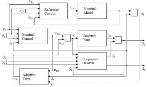
The proposed DMRAC based on cooperative observer with OCM is shown in Figure 1, that consists of two main blocks, namely a reference model and a main control system. The reference model generates a reference state $\left(x_{i, r}\right)$ which will be tracked by the estimated state $\left(\hat{x}_i\right)$. The main control system contains a nominal control signal ($u_{i, n}$) that utilizes the cooperative state estimation error and an adaptive term ($u_{i, a}$) that utilizes the nominal control signal ($u_{i, n}$), the estimated state ($\hat{x}_i$), the tracking error to the reference model ($e_i$). Nominal control is used to track the leader while adaptive term is used to depress the effect of uncertainty.
Figure 1. DMRAC based on cooperative observer
3.1 Controller design
The reference control signal is designed as:
$u_{i, r}=c_{2, i} K_i\left\{\sum_{j=1}^N a_{i j}\left(x_{j, r}-x_{i, r}\right)+g_{i i}\left(x_{0, r}-x_{i, r}\right)\right\}$ (11)
where, $c_{2, i}$ is a coupling gain, $K_i \in \mathbb{R}^{m \times n}$ is the feedback gain matrix which defined as:
$K_i=R_i^{-1} B_i^T P_{2, i}.$ (12)
Matrix $P_{2, i}$ is a solution of ARE.
$0=A_i{ }^T P_{2, i}+P_{2, i} A_i+Q_i-P_{2, i} B_i R_i{ }^{-1} B_i{ }^T P_{2, i}.$ (13)
The control input for each follower, Eq. (1), and cooperative observer, Eq. (7), which composed of a nominal control ($u_{i, n}$) and an adaptive term ($u_{i, a}$), is designed as:
$u_i=u_{i, n}-u_{i, a}.$ (14)
The nominal control input is designed as
$u_{i, n}=c_{2, i} K_i \hat{\varepsilon}_i$ (15)
with $K_i$ is as given by Eq. (12) and $\hat{\mathcal{E}}_i$ is cooperative tracking state estimation error that can be represented as:
$\hat{\varepsilon}_i=\sum_{i=1}^N a_{i j}\left(\hat{x}_j-\hat{x}_i\right)+g_{i i}\left(\hat{x}_0-\hat{x}_i\right)$. (16)
By following the procedure [20], the adaptive term is derived as by substituting Eq. (14) into Eq. (7), then adding and subtracting the term $c_{2, i} B_i K_i \hat{\varepsilon}_i$, finally yields:
$\begin{aligned} \dot{\hat{x}}_i=A_i \hat{x}_i & +B_i u_{i, n}-c_{1, i} F_i \psi_i +B_i \Omega_i\left[\theta_i^T \Phi_i\left(\sigma_i\left(\hat{x}_i\right), u_{i, n}\right)-u_{i, a}\right]\end{aligned}$ (17)
where,
$\theta_i^T=\left[\begin{array}{c}\Omega_i^{-1} W_i^T \\ I-\Omega_i^{-1}\end{array}\right]^T$ and $\Phi_i\left(\sigma_i\left(\hat{x}_i\right), u_{i, n}\right)=\left[\begin{array}{c}\sigma_i\left(\hat{x}_i\right) \\ u_{i, n}\end{array}\right]$ (18)
The adaptive term is constructed as:
$u_{i, a}=\hat{\theta}_i^T \Phi_i\left(\sigma_i\left(\hat{x}_i\right), u_{i, n}\right)$ (19)
where, $\hat{\theta}_i{ }^T$ is the estimated value of $\theta_i{ }^T$. For adaptation law, $\dot{\hat{\theta}}_i$, an optimal control modification [28] is adopted,
$\dot{\hat{\theta}}_i=\gamma_i \Phi_i\left(\sigma_i\left(\hat{x}_i\right), u_{i, n}, \psi_i\right)\left[e_i^T P_i\right.\left.+\mu_i \Phi_i^T\left(\sigma_i\left(\hat{x}_i\right), u_{i, n}, \psi_i\right) \hat{\theta}_i B_i^T P_i A_{i, m}{ }^{-1}\right] B_i$ (20)
where, $\gamma_i>0$ is the adaptation rate, $\mu_i>0$ is a positive weighting constant, while $e_i$ and $A_{i, m}$ will be defined later.
Remark 2: In order to realize the proposed control, it is assumed that full state information of the reference model is available or can be calculated. The reference states can be treated as virtual state references. All followers exchange information, to connected neighbors, that includes: estimation state ($\hat{x}_i$), and output estimation error ($\tilde{y}_i$). The reference model uses neighbors’ estimation state as neighbors’ reference states, i.e. $x_{0, r}=\hat{x}_{0, r}$ and $x_{j, r}=\hat{x}_j$. The leader sends its estimated state ($\hat{x}_0$), and output estimation error ($\tilde{y}_0$) to connected followers. It is assumed that $x_0=\hat{x}_0$ therefore $\tilde{y}_0=0$.
3.2 Tracking error dynamics of followers w.r.t the reference model
Since the observer guarantees $\hat{x}_i \rightarrow x_i$ as $\mathrm{t} \rightarrow \infty$ and the fact that $\hat{x}_j=x_{j, r}, \hat{x}_0=x_{0, r}$, therefore for the purpose of stability analysis, the tracking error of each follower w.r.t its reference model can be represented by $e_i=x_i-x_{i, r}$ which resulting the tracking error dynamics,
$\dot{e}_i=A_{i, m} e_i-B_i \Omega_i\left[\tilde{\theta}_i^T \Phi_i\left(\sigma_i\left(x_i\right), u_{i, n}\right)\right]$ (21)
with
$A_{i, m}=A_i-c_{2, i}\left(d_{i i}+g_{i i}\right) B_i K_i$. (22)
Here, $\theta_i=\hat{\theta}_i-\theta_i$ is the parameter estimation error and $\sigma_i\left(x_i\right)=x_i$ is the known basis function.
3.3 Tracking error dynamics of followers w.r.t the leader
Since the adaptive term suppresed the effects of uncertainties such that $x_i \rightarrow x_{i, r}$ as $t \rightarrow \infty$, therefore, for the purpose of stability analysis, the tracking error w.r.t the leader’s state can be expressed by using the reference model as:
$\rho_i=x_{i, r}-x_{0, r}$ (23)
where, $\rho_i=\left[\begin{array}{lll}\rho_{i, p} & \rho_{i, v} & \rho_{i, a}\end{array}\right]^T$ is the state tracking error to the leader. By following [10], since the leader has zero input which means that the leader moves at constant velocity $\left(\dot{v}_{0, r}=0\right)$, the tracking error of follower w.r.t the leader can be defined as:
$\left\{\begin{array}{c}\rho_{i, p}=p_{i, r}+i \cdot d_r-p_{0, r} \\ \rho_{i, v}=\dot{p}_{i, r}-\dot{p}_{0, r}=v_{i, r}-v_{0, r} . \\ \rho_{i, a}=\ddot{p}_{i, r}-\ddot{p}_{0, r}=a_{i, r}\end{array}\right.$ (24)
For the purpose of stability analysis, the control signal in Eq. (11) can be rewritten as:
$u_{i, r}=c_{2, i} K_i\left[\sum_{j=1}^N a_{i j}\left(\rho_j-\rho_i\right)-g_{i i} \rho_i\right]$ (25)
Therefore, the tracking error dynamics of each follower w.r.t the leader is represented as:
$\left\{\begin{array}{c}\dot{\rho}_{i, p}=\rho_{i, v} \\ \dot{\rho}_{i, v}=\rho_{i, a} \\ \dot{\rho}_{i, a}=-\frac{1}{\tau_i} \rho_{i, a}+\frac{1}{\tau_i} c_{2, i} K_i\left[\sum_{j=1}^N a_{i j}\left(\rho_j-\rho_i\right)\right]-g_{i i} \rho_i\end{array}\right]$ (26)
where, $K_i=\left[k_{i, p}, k_{i, v}, k_{i, a}\right]$. The global tracking error dynamics of vehicle platoon, Eq. (26), can be defined as:
$\dot{\rho}=\hat{A} \rho,$ (27)
where, $\rho=\left[\rho_p, \rho_v, \rho_a\right]^T$ with $\rho_\pi=\left[\rho_{1, \pi}, \rho_{2, \pi}, \ldots, \rho_{N, \pi}\right]^T$ for $\pi \in\{p, v, a\}$. Here,
$\hat{A}=\left[\begin{array}{ccc}0_N & I_N & 0_N \\ 0_N & 0_N & I_N \\ -\alpha_p H & -\alpha_v H & -\alpha_a H-\vartheta\end{array}\right]$, (28)
where, $\alpha_\pi=\operatorname{diag}\left(\alpha_{1, \pi}, \alpha_{2, \pi}, \ldots, \alpha_{N, \pi}\right)$ with $\alpha_{i, \pi}=\frac{1}{\tau_i} c_i k_{i, \pi}$ for $\pi \in\{p, v, a\}, \vartheta=\operatorname{diag}\left(\frac{1}{\tau_1}, \frac{1}{\tau_2}, \ldots, \frac{1}{\tau_N}\right)$ and $H=L+G$.
Theorem 1. Consider a vehicle platoon with network topology satisfying Assumption 1. Lead vehicle has dynamics as in Eq. (3), followers have dynamics as in Eq. (1) with the observer as in Eq. (7) with observer gain Fi as in Eq. (8) and reference model as in Eq. (10). If each follower applied a distributed controller, Eq. (14), with feedback gain Ki as in Eq. (12) and selecting $C_{2, i}$ such that:
$c_{2, i} \geq \frac{1}{2\left(d_{i i}+g_{i i}\right)}$ (29)
along with the adaptation law, Eq. (20), then it will result in stable and uniformly bounded tracking error w.r.t reference model, in compact set $\mathcal{C}$,
$\mathcal{C}=\left\{\tilde{\theta}_i^T \Phi_i\left(\sigma_i\left(x_i\right), u_{i, n}\right):\left\|\tilde{\theta}_i{ }^T \Phi_i\left(\sigma_i\left(x_i\right), u_{i, n}\right)\right\|>\beta\right.\left.=\frac{2 \bar{\sigma}\left(B_i{ }^T P_i A_{i, m}{ }^{-1} B_i\right)\left\|\theta_i \Phi_i\left(\sigma_i\left(x_i\right), u_{i, n}\right)\right\|}{\sigma\left(B_i^T A_{i, m}{ }^{-T} Q_i A_{i, m}{ }^{-1} B_i\right)}\right\}$ (30)
and guarantee the stability of vehicle platoon, Eq. (27). Here, $\underline{\sigma}\left({ }^.\right)$ and $\bar{\sigma}(\cdot)$ are the minimum and maximum singular values, respectively.
Proof. For stability proof, it will be shown that the tracking error w.r.t the reference model is uniformly bounded in compact set $\mathcal{C}$, and following by the stability of the closed loop dynamic, Eq. (27).
Proof of the uniformly bounded of ei.
Lyapunov candidate function is chosen as:
$V_i\left(e_i, \tilde{\theta}_i\right)=e_i^T P_i e_i+\gamma_i^{-1} \operatorname{tr}\left(\Omega_i^{\frac{1}{2}} \tilde{\theta}_i^T \tilde{\theta}_i \Omega_i^{\frac{1}{2}}\right)$. (31)
The first derivative of Eq. (31) along Eq. (21) yields:
$\dot{V}_i=e_i^T\left[P_i A_{i, m}+A_{i, m}{ }^T P_i\right] e_i-$
$2 e_i^T P_i B_i \Omega_i \tilde{\theta}_i^T \Phi_i\left(\sigma_i\left(x_i\right), u_{i, n}\right)+$
$2 \gamma^{-1} \operatorname{tr}\left(\Omega_i \tilde{\theta}_i^T \dot{\hat{\theta}}_i\right)$ (32)
Substituting Eq. (20) and re-arranging yields:
$\dot{V}_i=e_i^T\left[P_i A_{i, m}+A_{i, m}{ }^T P_i\right] e_i-$
$2 e_i^T P_i B_i \Omega_i \tilde{\theta}_i^T \Phi_i\left(\sigma_i\left(x_i\right), u_{i, n}\right)+$
$2 \operatorname{tr}\left(\Omega_i \tilde{\theta}_i^T \Phi_i\left(\sigma_i\left(x_i\right), u_{i, n}\right)\left\{e_i^T P_i B_i\right.\right.$
$\left.\left.+\mu_i \Phi_i^T\left(\sigma_i\left(x_i\right), u_{i, n}\right) \hat{\theta}_i B_i^T P_i A_{i, m}{ }^{-1} B_i\right\}\right)$ (33)
Using trace identity $\operatorname{tr}\left(a^T b\right)=b a^T$, Eq. (33) can be re-expressed as:
$\dot{V}_i=e_i{ }^T\left[P_i A_{i, m}+A_{i, m}{ }^T P_i\right] e_i-$
$2 e_i^T P_i B_i \Omega_i \tilde{\theta}_i{ }^T \Phi_i\left(\sigma_i\left(x_i\right), u_{i, n}\right)+$
$2\left\{e_i{ }^T P_i B_i+\mu_i \Phi_i{ }^T\left(\sigma_i\left(x_i\right), u_{i, n}\right) \hat{\theta}_i B_i{ }^T P_i A_{i, m}{ }^{-1} B_i\right\}$
$\Omega_i \tilde{\theta}_i{ }^T \Phi_i\left(\sigma_i\left(x_i\right), u_{i, n}\right)$ (34)
After some elimination, finally, it obtained that:
$\dot{V}_i=e_i^T\left[P_i A_{i, m}+A_{i, m}{ }^T P_i\right] e_i+$
$2 \mu_i \Omega_i \Phi_i^T\left(\sigma_i\left(x_i\right), u_{i, n}\right) \hat{\theta}_i B_i^T P_i A_{i, m}{ }^{-1} B_i$
$\tilde{\theta}_i^T \Phi_i\left(\sigma_i\left(x_i\right), u_{i, n}\right)$ (35)
It is known that $\theta_i+\tilde{\theta}_i=\hat{\theta}_i$, therefore Eq. (35) become:
$\dot{V}_i=e_i^T\left[P_i A_{i, m}+A_{i, m}{ }^T P_i\right] e_i+$
$2 \mu_i \Omega_i \Phi_i^T\left(\sigma_i\left(x_i\right), u_{i, n}\right) \theta_i B_i^T{ }^T P_i A_{i, m}{ }^{-1} B_i$
$\tilde{\theta}_i^T \Phi_i\left(\sigma_i\left(x_i\right), u_{i, n}\right)+2 \mu_i \Omega_i \Phi_i^T\left(\sigma_i\left(x_i\right), u_{i, n}\right) \tilde{\theta}_i$
$B_i{ }^T P_i A_{i, m}{ }^{-1} B_i \tilde{\theta}_i^T \Phi_i\left(\sigma_i\left(x_i\right), u_{i, n}\right)$ (36)
Consider the first term in Eq. (36), by substituting Eq. (22), $P_i A_{i, m}+A_{i, m}{ }^T P_i$ becomes:
$\begin{aligned} P_i A_{i, m}+A_{i, m}{ }^T P_i & =-Q_i-\left(2 c_{2, i}\left(d_{i i}+g_{i i}\right)\right. -1) K_i^T R_i K_i\end{aligned}$ (37)
Therefore, Eq. (36) becomes:
$\dot{V}_i=e_i^T\left[-Q_i-\left(2 c_{2, i}\left(d_{i i}+g_{i i}\right)-1\right) K_i^T R_i K_i\right] e_i$
$+2 \mu_i \Omega_i \Phi_i{ }^T\left(\sigma_i\left(x_i\right), u_{i, n}\right) \theta_i B_i P_i A_{i, m}{ }^{-1} B_i$
$\tilde{\theta}_i^T \Phi_i\left(\sigma_i\left(x_i\right), u_{i, n}\right)+2 \mu_i \Omega_i \Phi_i{ }^T\left(\sigma_i\left(x_i\right), u_{i, n}\right) \tilde{\theta}_i$
$B_i{ }^T P_i A_{i, m}{ }^{-1} B_i \tilde{\theta}_i^T \Phi_i\left(\sigma_i\left(x_i\right), u_{i, n}\right)$ (38)
Following [28, 30], it can be seen that the sign-definiteness of Eq. (38) is rely on the sign-defininiteness of $P_i A_{i, m}{ }^{-1}$. Where, the evaluation of sign-definiteness of $P_i A_{i, m}{ }^{-1}$ can be conducted by using the negative definite matrix property, i.e. "A general real matrix $M$ is negative definite if and only if its symmetric part $M_s=\frac{1}{2}\left(M+M^T\right)$ is also negative definite". Denote $M=P_i A_{i, m}{ }^{-1}$, then Eq. (37) can be pre and post multiplied by $\frac{1}{2} A_{i, m}{ }^{-T}$ and $A_{i, m}{ }^{-1}$, finally yields:
$\begin{aligned} & \frac{1}{2}\left(P_i A_{i, m}{ }^{-1}+A_{i, m}{ }^{-T} P_i\right)=-\frac{1}{2}\left[A_{i, m}{ }^{-T} Q_i A_{i, m}{ }^{-1}\right. \\ &+A_{i, m}{ }^{-T}\left(2 c_{2, i}\left(d_{i i}+g_{i i}\right)\right. \left.-1) K_i^T R_i K_i A_{i, m}{ }^{-1}\right]\end{aligned}$ (39)
By selecting a coupling gain $C_{2, i}$ that satisfies Eq. (29), the right-hand side of Eq. (39) is negative definite which mean that $M=P_i A_{i, m}^{-1}<0$. This matrix can be decomposed into the sum of a symmetric matrix Ms and an anti-symmetric matrix $N$, i.e. $M=M_s+N$, where $M_S=$ $\frac{1}{2}\left(P_i A_{i, m}{ }^{-1}+A_{i, m}{ }^{-T} P_i\right)$ and $N=\frac{1}{2}\left(P_i A_{i, m}{ }^{-1}-A_{i, m}{ }^{-T} P_i\right)$. By choosing y as a vector of matching dimensions, then pre and post multiplied $M=M_s+N$ by $y^T$ and y, considering that $N$ is anti-symmetric matrix such that $y^T N y=0$, finally yields:
$\begin{aligned} & y^T P_i A_{i, m}{ }^{-1} y=-\frac{1}{2} y^T\left[A_{i, m}{ }^{-T} Q_i A_{i, m}{ }^{-1}\right. +A_{i, m}{ }^{-T}\left(2 c_{2, i}\left(d_{i i}+g_{i i}\right)\right. \left.-1) K_i{ }^T R_i K_i A_{i, m}{ }^{-1}\right] y\end{aligned}$ (40)
Let choose $y=B_i \tilde{\theta}_i^T \Phi_i\left(\sigma_i\left(x_i\right), u_{i, n}\right)$, then Eq. (38) can be represented as:
$\dot{V}_i=e_i^T\left[-Q_i-\left(2 c_{2, i}\left(d_{i i}+g_{i i}\right)-1\right) K_i^T R_i K_i\right] e_i+2 \mu_i \Omega_i \Phi_i{ }^T\left(\sigma_i\left(x_i\right), u_{i, n}\right) \theta_i B_i{ }^T P_i A_{i, m}{ }^{-1} B_i$
$\tilde{\theta}_i^T \Phi_i\left(\sigma_i\left(x_i\right), u_{i, n}\right)-\mu_i \Omega_i \Phi_i{ }^T\left(\sigma_i\left(x_i\right), u_{i, n}\right) \tilde{\theta}_i B_i{ }^T$
$\left[A_{i, m}{ }^{-T} Q_i A_{i, m}{ }^{-1}+A_{i, m}{ }^T\left(2 c_{2, i}\left(d_{i i}+g_{i i}\right)\right.\right.-1) K_i^T R_i K_i A_{i, m}{ }^{-1}] B_i \tilde{\theta}_i^T \Phi_i\left(\sigma_i\left(x_i\right), u_{i, n}\right)$ (41)
By choosing a coupling gain $c_{2, i}$ that satisfies Eq. (29), the upper bound of $\dot{V}_i$ is:
$\dot{V}_i \leq-\underline{\sigma}\left(Q_i\right)\left\|e_i\right\|^2-\mu_i \Omega_i \underline{\sigma}\left(B_i{ }^T A_{i, m}{ }^{-T} Q_i A_{i, m}{ }^{-1} B_i\right)$
$\left\|\tilde{\theta}_i{ }^T \Phi_i\left(\sigma_i\left(x_i\right), u_{i, n}\right)\right\|^2$
$+2 \mu_i \Omega_i \bar{\sigma}\left(B_i{ }^T P_i A_{i, m}{ }^{-1} B_i\right)\left\|\theta_i \Phi_i\left(\sigma_i\left(x_i\right), u_{i, n}\right)\right\|$
$\left\|\tilde{\theta}_i{ }^T \Phi_i\left(\sigma_i\left(x_i\right), u_{i, n}\right)\right\|$ (42)
Thus, with:
$\left\|\tilde{\theta}_i^T \Phi_i\left(\sigma_i\left(x_i\right), u_{i, n}\right)\right\| \geq$
$\frac{2 \bar{\sigma}\left(B_i{ }^T P_i A_{i, m}{ }^{-1} B_i\right)\left\|\theta_i \Phi_i\left(\sigma_i\left(x_i\right), u_{i, n}\right)\right\|}{\sigma\left(B_i{ }^T A_{i, m}{ }^{-T} Q_i A_{i, m}{ }^{-1} B_i\right)}$ (43)
render $\dot{V}_i \leq 0$. Since,
$V_i(t \rightarrow \infty) \leq V_i(0)-\underline{\sigma}\left(Q_i\right) \int_0^{\infty}\left\|e_i\right\|^2 d t-$
$\mu_i \Omega_i \underline{\sigma}\left(B_i{ }^T A_{i, m}{ }^{-T} Q_i A_{i, m}{ }^{-1} B_i\right)$
$\int_0^{\infty}\left\|\tilde{\theta}_i^T \Phi_i\left(\sigma_i\left(x_i\right), u_{i, n}\right)\right\|^2 d t+$
$2 \mu_i \Omega_i \bar{\sigma}\left(B_i{ }^T P_i A_{i, m}{ }^{-1} B_i\right)$
$\int_0^{\infty}\left\|\theta_i \Phi_i\left(\sigma_i\left(x_i\right), u_{i, n}\right)\right\|\left\|\tilde{\theta}_i^T \Phi_i\left(\sigma_i\left(x_i\right), u_{i, n}\right)\right\| d t<\infty$ (44)
It means that $V_i(t \rightarrow \infty)<V_i(0)$, therefore $V_i$ decrease inside a compact set $\mathcal{C} \subset \mathbb{R}^n$ as described in Eq. (30). However, $V_i$ increase inside the complementary set $\mathcal{C}=$ $\left\{\left\|\tilde{\theta}_i{ }^T \Phi_i\left(\sigma_i\left(x_i\right), u_{i, n}\right)\right\| \in \mathbb{R}^n:\left\|\tilde{\theta}_i{ }^T \Phi_i\left(\sigma_i\left(x_i\right), u_{i, n}\right)\right\| \leq \beta\right\}$ which contain $\tilde{\theta}_i^T=0$ and will inside $\mathcal{C}$. By the LaSalle's extension of the Lyapunov method, $\tilde{\theta}_i$ is uniformly bounded. It implies that the tracking error $e_i$ is uniformly bounded.
Proof of the stability of $\dot{\rho}$.
Inspired by reference [10], stability analysis of the platoon can be conducted by using the characteristic equation of Eq. (27) as:
$\left|\lambda I_N-\hat{A}\right|=\left|\begin{array}{ccc}\lambda I_N & -I_N & 0_N \\ 0_N & \lambda I_N & -I_N \\ \alpha_p H & \alpha_v H & \lambda I_N+\alpha_a H+\vartheta\end{array}\right|$ (45)
$=\lambda^3 I_N+\lambda^2\left(\alpha_a H+\vartheta\right)+\lambda \alpha_v H+\alpha_p H$ (46)
Here, $\alpha_p, \alpha_v, \alpha_a, \vartheta$ are diagonal matrices and H is lower triangular matrix, therefore Eq. (46) can be described as:
$\begin{aligned}\left|\lambda I_N-\hat{A}\right|=\prod_{i=1}^N \lambda^3 & +\lambda^2\left[\alpha_{i, a}\left(d_{i i}+g_{i i}\right)+\frac{1}{\tau_i}\right] +\lambda\left[\alpha_{i, v}\left(d_{i i}+g_{i i}\right)\right]+\alpha_{i, p}\left(d_{i i}+g_{i i}\right)\end{aligned}$ (47)
The stability of the global tracking error dynamics Eq. (27) is equivalent to the stability of the following N characteristic equations,
$\lambda^3+\lambda^2\left[\alpha_{i, a}\left(d_{i i}+g_{i i}\right)+\frac{1}{\tau_i}\right]+\lambda\left[\alpha_{i, v}\left(d_{i i}+g_{i i}\right)\right]$
$+\alpha_{i, p}\left(d_{i i}+g_{i i}\right)=0, \quad i=1,2, \ldots, N$ (48)
Since H is lower triangular matrix, it is seen that $\hat{A}$ in Eq. (28) is composed of $A_i-c_{2, i}\left(d_{i i}+g_{i i}\right) B_i K_i$ which is equal to $A_{i, m}$ as in Eq. (22). From Eq. (37), by choosing the proper $c_{2, i}$ it shown that $A_{i, m}$ is Hurwitz for all $i$. Therefore, all the eigenvalues of Eq. (48) have negative real parts and guarantee stability of vehicle platoon.
This completes the proof.
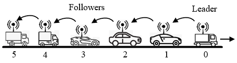
For numerical simulation analysis, a heterogeneous vehicle platoon consisted of 1-leader and 5-followers, formed based on PF topology and constant spacing policy with the desired inter-vehicular distance dr=5 m, is used, Figure 2.
Vehicles have nominal inertial time lags$\tau_0=0.6, \tau_1=0.25, \tau_2=0.27, \tau_3=0.3, \tau_4=0.5$ and $\tau_5=0.7$. Followers are subjected to uncertainty in the inertial time lag which represented by following constant weighting matrices: $W_1{ }^T=\left[\begin{array}{lll}0 & 0 & 0.286\end{array}\right], W_2{ }^T=\left[\begin{array}{lll}0 & 0 & 0.27\end{array}\right], W_3{ }^T=\left[\begin{array}{ll}0 & 0\end{array}\right.$ $0.926], W_4{ }^T=\left[\begin{array}{lll}0 & 0 & 0.286\end{array}\right]$ and $W_5{ }^T=\left[\begin{array}{lll}0 & 0 & 0.125\end{array}\right]$. The actual control effectiveness for followers is $\Omega_1=0.5, \Omega_2=0.6$, $\Omega_3=0.6, \Omega_4=0.7$ and $\Omega_5=0.7$. It is assumed that only position and velocity information can be obtained, therefore the output matrix is,
$C_i=\left[\begin{array}{lll}1 & 0 & 0 \\ 0 & 1 & 0\end{array}\right]$ (49)
The initial states of vehicles are as follows: $x_0(0)=$ $[60,20,0]^T, \quad x_1(0)=[40,18,0]^T, \quad x_2(0)=[25,19,0]^T$, $x_3(0)=[17,22,0]^T, \quad x_4(0)=[10,21,0]^T \quad$ and $x_5(0)=$ $[0,17,0]^T$, while the initial state of the estimated state are selected near the initial states, namely $\hat{x}_1(0)=[38,17,0]^T$, $\hat{x}_2(0)=[27,18,0]^T \quad, \quad \hat{x}_3(0)=[16,23,0]^T \quad, \quad \hat{x}_4(0)=$ $[12,22,0]^T$ and $\hat{x}_5(0)=[2,16,0]^T$.
The coupling gains for the observer and nominal controls, the adaptation rates and the weighting constant are selected to be the same for each follower, namely $c_{1, i}=0.1$ and $c_{2, i}=$ $0.5, \gamma_i=1$ and $\mu_i=0.2$ respectively. While the observer gain, $F_i$, and the feedback gain, $K_i$ are obtained according to Eq. (8) and Eq. (12) respectively by selecting $Q_i=I_{3 \times 3}$ and $R_j=0.1$.
Remark 3: In practice, the control parameters that require tuning are $Q_i, R_i, c_{1, i}, c_{2, i}, \gamma_i$ and $\mu_i$. It should be noted that the choice of $Q_i, R_i, c_{1, i}$ and $c_{2, i}$, values is a trade-off between consensus tracking performance and a reasonable control signal. The larger the value of $Q_i, c_{1, i}$ and $c_{2, i}$, the better the consensus tracking performance, conversely, the smaller the value of $R_i$, the better the consensus tracking performance. However, the increase in performance will be followed by an increase in the control signal [22]. The higher the adaptation rate, $\gamma_i$, the faster the follower can track to reference model, but it is followed by the possibility of high-frequency oscillations of the control signal [23]. The greater the value of $\mu_i$, the greater the frequency attenuation of the control signal.
Figure 2. A vehicle platoon with PF topology [22]
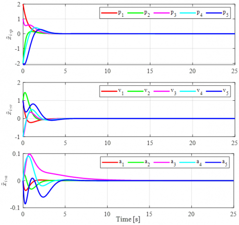
Figure 3. The state estimation error, $\hat{x}_i$
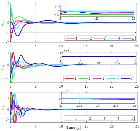
Figure 4. Tracking error with respect of reference model, $e_i$
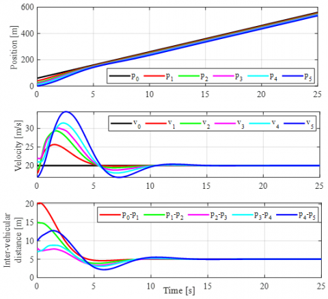
Figure 5. Synchronization of the platoon
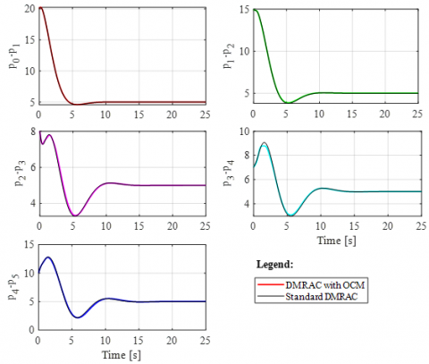
Figure 6. Inter-vehicular distance comparison between the proposed DMRAC with OCM and the standard DMRAC
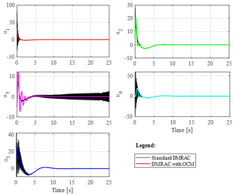
Figure 7. Control input comparison between proposed DMRAC and standard DMRAC
Table 1. Tracking error w.r.t the reference model
|
Tracking error (t≥20s) |
Min |
Max |
|
Distance [m] |
-0.026 |
0.006 |
|
Velocity [m/s] |
-0.0003 |
-0.0001 |
|
Acceleration [m/s2] |
-0.00007 |
-0.00004 |
Numerical simulations show that the state estimation error is approach zero as time approach infinity, Figure 3. While, in Figure 4, it is shown that the tracking error of followers w.r.t the reference model is bounded in some constant values, Table 1. Stability and synchronization of the heterogeneous vehicle platoon is shown in Figure 5. It is seen that followers able to keep the inter-vehicular distance as required, with small bounded residual error, namely $\pm$ 0.025 m.
For further analysis, the results were compared with the standard DMRAC [22] which was modified to be designed based on the cooperative observer and applied to heterogeneous vehicle platoons (standard DMRAC). Here, the inter-vehicular distance for both schemes is analyzed for each follower as shown in Figure 6. It can be seen that the performance of the proposed controller is relatively the same with standard DMRAC, however the proposed controller able to eliminate high frequency oscillation in the control input which occurred in the standard DMRAC, Figure 7. This control signal improvements have implications for significant improvements in vehicle jerks and driving comfort, since the control input represents the desired acceleration of the vehicle. Moreover, with smooth trajectory control input, it will improve energy efficiency.
This paper presented a distributed model reference adaptive control based on cooperative observer for synchronization of heterogeneous vehicle platoon. The control scheme utilized a reference model and a main control system. The reference model generated a reference state that will be tracked by the estimated state which provided by the cooperative observer. The main control system consisted of two terms, namely (i) a nominal control that utilized the cooperative state estimation error and (ii) an adaptive term that adopted optimal control modification. Through stability analysis and numerical simulation, it is shown that the state estimation error approach zero as time approach infinity. Moreover, it shown that the tracking error w.r.t the reference state is bounded in some small constant values which implied that the follower synchronized the leader state with small residual error. The proposed control exhibited the advantage of eliminating high frequency oscillation in the control input which usually occurred in the standard DMRAC with high adaptation rate. This paper still assumes that the leader moves at constant velocity and communication between vehicles is in ideal conditions. Therefore, future works may focus on several implementation issues such as explicitly considering poor communication problems in controller design and stability analysis and on the case that lead vehicle has possibility to move at time-varying velocity.
[1] Bouradi, S., Negadi, K., Araria, R., Boumediene, B., Koulali, M. (2022). Design and implementation of a four-quadrant DC-DC converter based adaptive fuzzy control for electric vehicle application. Mathematical Modelling of Engineering Problems, 9(3): 721-730. https://doi.org/10.18280/mmep.090319
[2] Elliot, D., Keen, W., Miao, L. (2019). Recent advances in connected and automated vehicles. Journal of Traffic and Transportation Engineering, 6(2): 109-131. https://doi.org/10.1016/j.jtte.2018.09.005
[3] Tho, Q.H., Phap, H.C., Phuong, P.A. (2022). Motion planning solution with constraints based on minimum distance model for lane change problem of autonomous vehicles. Mathematical Modelling of Engineering Problems, 9(1): 251-260. https://doi.org/10.18280/mmep.090131
[4] Subotić, M., Softić, E., Radičević, V., Bonić, A. (2022). Modeling of operating speeds as a function of longitudinal gradient in local conditions on two-lane roads. Mechatronics and Intelligent Transportation Systems, 1(1): 24-34. https://doi.org/10.56578/mits010104
[5] Li, Y.X., Zhu, X.Y. (2022). Design and testing of cooperative motion controller for UAV-UGV system. Mechatronics and Intelligent Transportation Systems, 1(1): 12-23. https://doi.org/10.56578/mits010103
[6] Li, S.E., Zheng, Y., Li, K., Wang, J. (2015). An overview of vehicular platoon control under the four-component framework. IEEE Intelligent Vehicles Symposium (IV), Seoul, Korea (South), pp. 286-291. https://doi.org/10.1109/IVS.2015.7225700
[7] Hu, J., Bhowmick, P., Arvin, F., Lanzon, A., Lennox, B. (2020). Cooperative control of heterogeneous connected vehicle platoons: an adaptive leader-following approach. IEEE Robotics and Automation Letters, 5(2): 977-984. https://doi.org/10.1109/LRA.2020.2966412
[8] Zheng, Y., Li, S.E., Wang, J., Cao, D., Li, K. (2016). Stability and scalability of homogeneous vehicular platoon: Study on the influence of information flow topologies. IEEE Transactions on Intelligent Transportation Systems, 17(1): 14-26. https://doi.org/10.1109/TITS.2015.2402153
[9] Gao, F., Li, S.E., Zheng, Y., Kum, D. (2016). Robust control of heterogeneous vehicular platoon with uncertain dynamics and communication delay. IET Intelligent Transport Systems, 10(7): 503-513. https://doi.org/10.1049/iet-its.2015.0205
[10] Zheng, Y., Bian, Y., Li, S., Li, S.E. (2021). Cooperative control of heterogeneous connected vehicles with directed acyclic interactions. IEEE Intelligent Transportation Systems Magazine, 13(2): 127-141. https://doi.org/10.1109/MITS.2018.2889654
[11] Zegers, J.C., Semsar-Kazerooni, E., Ploeg, J., Van De Wouw, N., Nijmeijer, H. (2016). Consensus-based bi-directional CACC for vehicular platooning. 2016 American Control Conference (ACC), Boston, pp. 2578-2584. https://doi.org/10.1109/ACC.2016.7525305
[12] Harfouch, Y.A., Yuan, S., Baldi, S. (2018). An adaptive switched control approach to heterogeneous platooning with intervehicle communication losses. IEEE Transactions on Control of Network Systems, 5(3): 1434-1444. https://doi.org/10.1109/TCNS.2017.2718359
[13] Wang, C., Gong, S., Zhou, A., Li, T., Peeta, S. (2019). Cooperative adaptive cruise control for connected autonomous vehicles by factoring communication-related constraints. Transportation Research Part C: Emerging Technologies, 113: 124-145. https://doi.org/10.1016/j.trc.2019.04.010
[14] Zhang, Y., Wang, M., Hu, J., Liberis, N.B. (2020). Semi-constant spacing policy for leader-predecessor-follower platoon control via delayed measurements synchronization. IFAC-PapersOnLine, 53(2): 15096-15103. https://doi.org/10.1016/j.ifacol.2020.12.2032
[15] Yan, M., Song, J., Yang, P., Zuo, L. (2018). Neural adaptive sliding-mode control of a bidirectional vehicle platoon with velocity constraints and input saturation. Complexity. https://doi.org/10.1155/2018/1696851
[16] di Bernardo, M., Salvi, A., Santini, S. (2015). Distributed consensus strategy for platooning of vehicles in the presence of time-varying heterogeneous communication delays. IEEE Transactions on Intelligent Transportation Systems, 16(1): 102-112. https://doi.org/10.1109/TITS.2014.2328439
[17] Yucelen, T., Johnson, E.N. (2013). Control of multivehicle systems in the presence of uncertain dynamics. International Journal of Control, 86(9): 1540-1553. https://doi.org/10.1080/00207179.2013.790077
[18] Peng, Z., Wang, D., Zhang, H., Sun, G., Wang, H. (2013). Distributed model reference adaptive control for cooperative tracking of uncertain dynamical multi-agent systems. IET Control Theory & Applications, 7(8): 1079-1087. https://doi.org/10.1049/iet-cta.2012.0765
[19] Song, X., Chen, L., Wang, K., He, D. (2020). Robust time-delay feedback control of vehicular cacc systems with uncertain dynamics. Sensors, 20: 1775. https://doi.org/10.3390/s20061775
[20] Prayitno, A., Nilkhamhang, I. (2021). Distributed model reference adaptive control for vehicle platoons with uncertain dynamics. Engineering Journal, 25(8): 173-185. https://doi.org/10.4186/ej.2021.25.8.173
[21] Wang, C., Nijmeijer, H. (2015). String stable heterogeneous vehicle platoon using cooperative adaptive cruise control. 2015 IEEE 18th International Conference on Intelligent Transportation Systems, Gran Canaria, Spain, pp. 1977-1982. https://doi.org/10.1109/ITSC.2015.320
[22] Prayitno, A., Nilkhamhang, I. (2022). Synchronization of heterogeneous vehicle platoons using distributed model reference adaptive control. 2022 61st Annual Conference of the Society of Instrument and Control Engineers (SICE), Japan, pp. 295-300. https://doi.org/10.23919/SICE56594.2022.9905763
[23] Nguyen, N.T. (2018). Model-reference adaptive control. In Model-Reference Adaptive Control, Springer International Publishing AG 2018, (pp. 83-123). https://doi.org/10.1007/978-3-319-56393-0
[24] Bae, I., Moon, J., Seo, J. (2019). Toward a comfortable driving experience for a self-driving shuttle bus. Electronics, 8(9): 943. https://doi.org/10.3390/electronics8090943
[25] Burken, J., Nguyen, N., Griffin, B. (2010). Adaptive flight control design with optimal control modification for F-18 aircraft model. In AIAA Infotech@ Aerospace 2010, Atlanta, Georgia, pp. 3364. https://doi.org/10.2514/6.2010-3364
[26] Zhang, H., Lewis, F.L., Das, A. (2011). Optimal design for synchronization of cooperative systems: state feedback, observer and output feedback. IEEE Transactions on Automatic Control, 56(8): 1948-1952. https://doi.org/10.1109/TAC.2011.2139510
[27] Lewis, F.L., Zhang, H., Movric, K.H., Das, A. (2014). Cooperative control of multi-agent systems optimal and adaptive design approach. Springer-Verlag London. https://doi.org/10.1007/978-1-4471-5574-4
[28] Nguyen, N.T. (2012). Optimal control modification for robust adaptive control with large adaptive gain. Systems & Control Letters, 61(8): 485-494. https://doi.org/10.1016/j.sysconle.2012.01.009
[29] Zhang, H., Lewis, F.L. (2012). Adaptive cooperative tracking control of higher-order nonlinear systems with unknown dynamics. Automatica, 48(7): 1432-1439. https://doi.org/10.1016/j.automatica.2012.05.008
[30] Pacheco, A.M. (2018). Time delay margin analysis for model reference adaptive flight control laws: A bounded linear stability approach and application to aeroservoelasticity models. Master of Science Thesis. TU Delft Mechanical, Maritime and Materials Engineering, Delft University of Technology, Netherlands.