Widowati* | Sutrisno | Priyo Sidik Sasongko | Melvin Brilliant | Eka Triyana
© 2022 IIETA. This article is published by IIETA and is licensed under the CC BY 4.0 license (http://creativecommons.org/licenses/by/4.0/).
OPEN ACCESS
A virus that attacks the human respiratory system that first appeared in the province of Wuhan, China is known as COVID-19 (SARS COV2 n-corona virus). In order to anticipate the increasing of the cases, a strategy is needed to inhibit its growth and spread. Seeing the projection of future situations becomes very important, so we can anticipate with a selection of policy scenarios. The dynamical system model approach is very important for predicting future situations as well as selectable scenarios based on simulation results. In this study, we develop a COVID-19 transmission model which can be used to predict the epidemiological outcome and simultaneously to evaluate the effect of quarantine and hospitalization to COVID-19 spread. The mathematical model of the transmission of COVID-19 was developed in the form of the non-linear differential equation system, with seven variables, namely susceptible, exposed, infected, quarantined-1 (exposed individuals who were quarantined), quarantined-2 (infected individuals who were quarantined), hospitalized and recovered. The proposed model has a non-endemic and endemic equilibrium point. Local stability analysis of the non-endemic equilibrium point was investigated using the Routh-Hurwitz criterion, while global stability of the endemic equilibrium point was analyzed by using the Lyapunov method. If the basic reproduction number is less than one, then non-endemic equilibrium point is stable. On the other hand, if the basic reproduction number is greater than one, then endemic equilibrium point is stable. Verification of the developed model was carried out through numerical simulations using data from Central Java Province, Indonesia. We have investigated that parameter related to quarantine and hospitalize affect the number of new infections COVID-19 and the basic reproduction number. From the simulation results, it was found that strict quarantine and hospitalize have the potential to succeed in reducing and inhibiting the transmission of the COVID-19. It can be used by the government in making policies to increase the implementation of quarantine and hospitalize in the community.
mathematical modeling, stability analysis, Lyapunov method, endemic, quarantine, hospitalize, COVID-19
Coronavirus is a virus characterized by a crown of spikes on its surface. The most dangerous corona viruses today are MERS-CoV and SARS-CoV, which are the cause of severe diseases, such as MERS and SARS [1, 2]. At the end of 2019, in Wuhan, China, a epidemiological outbreak of COVID-19 caused by SARS-CoV appeared [3-5]. Upon further investigation, it was found that the disease was caused by infection with a new type of virus belonging to the coronavirus family, which was later named 2019 novel Coronavirus (2019-nCoV) [6]. World Health Organization (WHO) named the new virus SARS-CoV-2 (Severe Acute Respiratory Syndrome Coronavirus2) and the name of the disease was COVID-19 (Coronavirus Disease 2019) [7].
Following WHO advice to limit, control, delay and reduce the spread of COVID-19. To overcome this pandemic situation, various countries, including Indonesia, have implemented a quarantine system to reduce the transmission rate of COVID-19. The Indonesian government has implemented several policies to reduce the transmission of the virus. Large-Scale Social Restrictions (PSBB) are a type of implementation of health quarantine in the region, in addition to regional quarantine, hospital quarantine, and self-quarantine. Community responses related to community health and social measures implemented by the federal government in order to reduce the spread of Covid-19 during a pandemic have been studied by Okafor et al. [8].
In the COVID-19 pandemic situation, in addition to the development of medical and medical science which has a major role in overcoming COVID-19, other fields of science that also have an important role in dealing with COVID-19, one of which is the field of mathematics, namely mathematical modeling. According to reference [9], mathematical modeling is a field of mathematics to represent the problems in the real-world into mathematical language, so that a more precise understanding of real-world problems is obtained. Mathematical modeling, through differential equations, can be applied to represent the phenomenon of change, one of which is in the field of biology, including the field of Health [10, 11].
In various cases of coronavirus disease spread, the epidemic model used to represent epidemic phenomena in a population. Several mathematical and statistical models have been developed by researchers. Adedotun [12] has been published the classification and regression tree models and also autoregressive integrated moving averages that are used for modeling and forecasting the confirmed COVID-19 cases.
Further, dynamical models of the COVID-19 spread, such as Suspected, Infected, and Removed (SIR) [13] and Suspected, Exposed, Infected, and Removed (SEIR) models [14] have been published to analyze the transmission between its subpopulations. SEIR is a modified model of the SIR model that has been presented in many reports, see e.g. [15-17]. Then, Tchoumi et al. [18] has modified the SIR model of two-strain COVID-19 transmission dynamics with strain one vaccination. Development of this compartmental model of the COVID-19 epidemic by adding Hospitalized subpopulation (SEIHR) has been investigated by Rahman et al. [19]. This model was built using a non-linear system of differential equations to predict the transmission of COVID-19. Furthermore, various studies about COVID-19 spread analysis using dynamical systems are also available in the literature, which were used to determine the effectiveness of treatments to prevent the transmission of the virus (see e.g. [20-26]). We summarize the specification of each developed model as well as the proposed model in this paper in Table 1. It shows the progress of the COVID-19 transmission model development extracted from published papers including the model developed in our study based on the divided compartments which represent the number of dependent variables from the dynamical model. Moreover, each model has its own uniqueness in term of the parameters involved in the model.
Table 1. Variables studied in the compartmental models of the COVID-19 transmission
(S: Suspectible; V: Vaccinated; E/L: Exposed/Laten;Q: Quarantined; I: Infected ; A: Asymptomatic ; H: Hospitalized; R: Recovered ; D: Death/Deceased body)
|
Source |
Compartments (Variables) |
||||||||
|
S |
V |
E/L |
Q |
I |
A |
H |
R |
D |
|
|
Mackolil and Mahanthesh [13] |
√ |
|
|
|
√ |
|
|
√ |
|
|
Parsamanesh et al. [17] |
√ |
√ |
|
|
√ |
|
|
|
|
|
Bärwolff et al. [27] |
√ |
|
|
|
√ |
|
|
√ |
|
|
Zewdie and Gakkha [28] |
√ |
|
|
|
√ |
|
|
√ |
√ |
|
Din et al. [14] |
√ |
|
√ |
|
√ |
|
|
√ |
|
|
Carcione et al. [15] |
√ |
|
√ |
|
√ |
|
|
√ |
|
|
Santoro et al. [16] |
√ |
|
√ |
|
√ |
|
|
√ |
|
|
Radha and Balamuralitharan [21] |
√ |
|
√ |
|
√ |
|
|
√ |
|
|
Cullenbine et al. [26] |
√ |
|
√ |
|
√ |
|
|
√ |
|
|
Yang and Wang [29] |
√ |
|
√ |
|
√ |
|
|
√ |
|
|
Ishtiaq [30] |
√ |
|
√ |
|
√ |
|
|
√ |
|
|
Schecter [31] |
√ |
|
√ |
|
√ |
|
|
√ |
|
|
Masoumnezhad et al. [20] |
√ |
√ |
|
|
√ |
|
|
√ |
|
|
Tchoumi et al. [18] |
√ |
√ |
|
|
√ |
|
|
√ |
|
|
Telles et al. [2] |
√ |
|
√ |
√ |
|
|
√ |
|
|
|
Lamichhane et al. [32] |
√ |
|
√ |
|
√ |
√ |
|
√ |
|
|
Hu et al. [25] |
√ |
|
√ |
√ |
√ |
|
|
√ |
|
|
Rahman et al. [19] |
√ |
|
√ |
|
√ |
|
√ |
√ |
|
|
Ala’raj et al. [12] |
√ |
|
√ |
|
√ |
|
√ |
|
√ |
|
Arin and Portet [1] |
√ |
|
√ |
|
√ |
√ |
|
√ |
|
|
Serhani and Labbardi [22] |
√ |
|
|
√ |
√ |
√ |
|
√ |
√ |
|
This paper |
√ |
|
√ |
√ |
√ |
|
√ |
√ |
|
Furthermore, policies are needed to anticipate an increase in cases, slow or stop the spread of the virus. By identifying the right policies to implement. The model of dynamical system model approach is very important to predict future conditions from the simulation results as well as the scenarios that can be selected. Analysis of the interaction between the most influential variables can help determine the sensitivity of the related parameters. This is done to determine the behavior of the system around the non-endemic and endemic equilibrium points. In this study, we formulated the COVID-19 spread model by considering the policies such as quarantine and hospital treatment. Therefore, there are new information and parameters involved in our proposed model so that it becomes the novelty in this work.
This paper is structured as follows: In the introduction, we describe the scientific background, importance, and objectives of this research. The mathematical formulation of COVID-19 spread, positivity and boundedness of solutions, and the basic reproduction number are discussed in the second section. In the third section, we propose the non-endemic and endemic equilibrium points. Stability analysis is discussed in the fourth section. Further, in the fifth section, numerical simulations based on data from Central Java Province Indonesia are demonstrated to verify the developed dynamical model. Finally in the sixth section, conclusions for the research are given.
The spread of COVID-19 model in this study, represents the interaction between seven subpopulations, that is namely susceptible (S), exposed (E), infected (I), quarantined-1 (Q1), quarantined-2 (Q2), hospitalized (H) and recovered (R). Hence, the total population at time t is represented by
$N(t)=S(t)+E(t)+I(t)+Q_1(t)+Q_2(t)+H(t)+R(t)$
In this model the migration rate is ignored. The transmission of COVID-19 is assumed from susceptible individuals (S) who are in contact with exposed individuals (E) and infected individuals (I) with the incidence rate $\beta_1$ and $\beta_2$ respectively. It is assumed that the exposed individuals (E) are transmitted to infected individuals (I) and the quarantined exposed individuals (Q1) is transmitted to quarantined infected individuals (Q2) with the same average rate of v, also the infected individuals (I) and the quarantined infected (Q2) are transmitted to hospitalized individuals (H) with the same transition rate of η. Hospitalized individuals (H) are transmitted to recovered individuals with rate of $\gamma$. The proposed COVID-19 disease transmission model is given in the scheme showed in Figure 1.
Figure 1. Schematic model of the spread of COVID-19
The dynamics of each compartment, which were used to formulate the mathematical model representing the COVID-19 spread, are described as follows. Changes in the susceptible individuals (S) cover: (1) increment due to the recruitment rate of A, (2) decrement due to infections from direct interactions between vulnerable individuals and COVID-19 carriers, and move to individuals E with rates $\beta_1$ and $\beta_2$, (3) decrement due to natural death by μ1, Further, it increased due to the rate of development from Q1 to S of $\varepsilon$.
The number of individuals in the exposed subpopulation (E) increased due to the interaction between susceptible individuals and COVID-19 carriers, causing E and I with rate $\beta_1$ and $\beta_2$ respectively. Further, it decreased due to the rate of development from E to Q1 and I of q1 and v respectively. Finally, there is a natural death of μ1.
Changes in the number of the exposed individual who were quarantined (Q1) cover: (1) increment due to the rate of development of exposed E to Q1 by the rate of q1, (2) decrement due to recovery with the rate of $\varepsilon$, (3) decrement due to the rate of transmission from Q1 to Q2 and natural death of v and μ1respectively.
The number of the infected individuals (I) increased due to the rate of development from the E class to positive individuals I by the rate of v. The infected individuals by COVID-19 decreased due to the rate of change of infected individuals to quarantine Q2 and hospitalized H by q2 and η respectively, decrement because of the death rate due to COVID-19 infected and natural deaths with the rate of μ2 and μ1 respectively.
Changes in the number of the infected individual who were quarantined (Q2) cover: (1) increment due to the rate of development of infected individuals I to Q2 and the rate of transmission from Q1 to Q2 by the rate of q2 and v respectively, (2) decrement because of the death rate due to COVID-19 infected and natural deaths with the rate of μ2 nd μ1 respectively. (3) decrement due to the rate of transmission from Q2 to H of $\eta$.
The number of the hospitalized individuals (H) increased by subpopulation transmissions from Q2 and I with the rate of $\eta$ Further, H reduced due to COVID-19 infected and natural deaths with the rate of μ2 and μ1 respectively. Finally, decrement due to the rate of transmission from H to R of $\gamma$.
The number of the recovered individual (R) increased by population transmissions from H with the rate of $\gamma$ and reduced due to natural deaths by μ1.
There are seven variables involved in the model, the dynamic of each variable is modeled as a differential equation. Below, we present the derivation of the differential equation of S only, where the model derivation for the other six variables was derived analogously. The dynamic of S at a time t with the time increment $\Delta t$ is modeled as follows:
$\begin{matrix} S(t+\Delta t)-S(t)=(A+\varepsilon {{Q}_{1}}(t)-{{\beta }_{1}}S(t)I(t) \\ -{{\beta }_{2}}S(t)E(t)-{{\mu }_{1}}S(t))\Delta t. \\ \end{matrix}$
By taking the limit value of S for $\Delta t \rightarrow 0$, we derive the following differential equation:
$\lim _{\Delta t \rightarrow 0} \frac{S(t+\Delta t)-S(t)}{\Delta t}=\frac{d S}{d t}=A+\varepsilon Q_1(t)-\beta_1 S(t) I(t)-\beta_2 S(t) E(t)-\mu_1 S(t)$.
Based on the dynamics described above and Figure 1, the non-linear differential equation system for all seven variables as the complete mathematical model of the transmission of COVID-19 disease is obtained as follows
$\left\{\begin{array}{l}\frac{d S}{d t}=A+\varepsilon Q_1-\beta_1 S I-\beta_2 S E-\mu_1 S, \\ \frac{d E}{d t}=\beta_1 S I+\beta_2 S E-q_1 E-\mu_1 E-v E, \\ \frac{d I}{d t}=v E-q_2 I-\eta I-\left(\mu_1+\mu_2\right) I, \\ \frac{d Q_1}{d t}=q_1 E-\varepsilon Q_1-v Q_1-\mu_1 Q_1, \\ \frac{d Q_2}{d t}=q_2 I+v Q_1-\eta Q_2-\left(\mu_1+\mu_2\right) Q_2, \\ \frac{d H}{d t}=\eta I+\eta Q_2-\gamma H-\left(\mu_1+\mu_2\right) H, \\ \frac{d R}{d t}=\gamma H-\mu_1 R.\end{array}\right.$ (1)
with non-negative initial values
$S(0)=S_0, \quad E(0)=E_0, I(0)=I_0, Q_1(0)=Q_{1_0}, Q_2(0)=Q_{2_0}, H(0)=H_0, R(0)=R_0$
and all parameters are positive.
2.1 Positiveness and boundedness of solutions
In order to analyze whether the COVID-19 model as in (1) has epidemic significance, the first step is to prove that the variables are positive. This means that the solution of the system of equations with non-negative initial conditions must be positive for every t>0 and also model (1) represent the interaction between of human subpopulations, so the solutions are bounded. The next theorem has guaranteed the positiveness and boundedness of solutions of the system.
Theorem 1. Let S(0)≥0, E(0)≥0, I(0)≥0, Q1(0)≥0, Q2(0)≥0,, H(0)≥0, and R(0)≥0, then the solutions S(t), E(t), I(t), Q1(t), Q2(t), H(t),and R(t) of the model (1) are positive for every t>0.
Proof. Please see Appendix A for proof
Theorem 2. The feasible region of the model (1) is defined by $\Omega=\left\{\left(S(t), E(t), I(t), Q_1(t), Q_2(t), H(t), R(t)\right) \in\right.\left.\mathbb{R}_{+}^7: 0 \leq N(t) \leq \frac{A}{\mu_1}\right\}$ is positively invariant for the system (1).
Proof. Please see Appendix B for proof
2.2 The basic reproductive number
The basic reproductive number ($\mathfrak{N}_0$) is the average number of new infection cases in a population. If $\mathfrak{N}_0<1$, the spread of the disease can be controlled and will not become an epidemic [27, 28]. However, if $\mathfrak{N}_0<1$, then each infected individual will spread the disease to other individuals, so that it can lead to an epidemic [29, 30]. The reproduction number is found from the Next Generation Matrix (NGM) method, which is to build a matrix that generates the number of infected individuals [31] in this dynamic system model the infected compartments are the exposed (E) and infectious (I).
For example, $X=\left[\begin{array}{ll}E & I\end{array}\right]^T$ so that it can be written as
$\frac{d X}{d t}=F(X)-V(X)=\left[\begin{array}{c}\beta_1 S I+\beta_2 S E-q_1 E-\mu_1 E-v E \\ v E-q_2 I-\eta I-\left(\mu_1+\mu_2\right) I\end{array}\right]$
where, F(x) is a matrix containing the initial infection rate, while V(x) is a matrix containing the rate of movement of the infected population, with the values of F(x) and V(x) being
$F(X)=\left[\begin{array}{l}F_1 \\ F_2\end{array}\right]=\left[\begin{array}{c}\beta_1 S I+\beta_2 S E \\ 0\end{array}\right]$,
and
$V(X)=\left[\begin{array}{l}V_1 \\ V_2\end{array}\right]=\left[\begin{array}{c}q_1 E+\mu_1 E+v E \\ q_2 I+\eta I+\left(\mu_1+\mu_2\right) I-v E\end{array}\right]$
Suppose F and V are Jacobian matrices of F(x) and V(x) and substitute the value of the variable with the equilibrium point $K^0\left(S^0, E^0, I^0, Q_1^0, Q_2^0\right)=\left(\frac{A}{\mu_1}, 0,0,0,0\right)$ then we get:
$F=\left[\begin{array}{ll}\frac{\partial F_1}{\partial E} & \frac{\partial F_1}{\partial I} \\ \frac{\partial F_2}{\partial E} & \frac{\partial F_2}{\partial I}\end{array}\right]=\left[\begin{array}{cc}\beta_2 S & \beta_1 S \\ 0 & 0\end{array}\right]=\left[\begin{array}{cc}\frac{\beta_2 A}{\mu_1} & \frac{\beta_1 A}{\mu_1} \\ 0 & 0\end{array}\right]$,
and
$V=\left[\begin{array}{cc}\frac{\partial V_1}{\partial E} & \frac{\partial V_1}{\partial I} \\ \frac{\partial V_2}{\partial E} & \frac{\partial V_2}{\partial I}\end{array}\right]=\left[\begin{array}{cc}q_1+\mu_1+v & 0 \\ -v & q_2+\eta+\mu_1+\mu_2\end{array}\right]$
Furthermore, to determine the inverse of the V method is used Next Generation Matrix (NGM)
$V^{-1}=\frac{1}{\operatorname{det}(V)} \operatorname{Adj}(V)$
$V^{-1}=\frac{1}{q_1+\eta+\mu_1+\mu_2}\left[\begin{array}{cc}q_1+\eta+\mu_1+\mu_2 & 0 \\ v & q_1+\mu_1+v\end{array}\right]$.
So that the inverse matrix V, as follows
$N G M=F(V)^{-1} N G M\left[\frac{\beta_2 A}{\mu_1\left(q_1+\mu_1+v\right)}+\frac{\beta_1 A v}{\mu_1\left(q_1+\mu_1+v\right)\left(q_2+\eta+\mu_1+\mu_2\right)} \frac{\beta_1 A}{\mu_1\left(q_2+\eta+\mu_1+\mu_2\right)}\right]$
The reproduction number is ($\mathfrak{R}_0$) obtained from the radius spectral of the NGM determined using a non-endemic equilibrium point. The reproduction number obtained are as follow
$\Re_0=\frac{\beta_2 A}{\mu_1\left(q_1+\mu_1+v\right)}+\frac{\beta_1 A v}{\mu_1\left(q_1+\mu_1+v\right)\left(q_2+\eta+\mu_1+\mu_2\right)}$.
The form $\mathfrak{R}_0$ above, it shows that the parameters q1 and q2 relating to quarantine and also η (transition rate from quarantined and infected individuals to hospitalized individuals) are inversely proportional to the value of the basic reproduction number which will determine the type of stability. The greater the value of $q_1, q_2$ and $\eta$, will impact the smaller the value of $\mathfrak{R}_0$. This parameter makes an important contribution to the occurrence of epidemics when the system has an endemic equilibrium and determines the speed in achieving COVID-19 disease-free equilibrium when $\mathfrak{R}_0$ is less than one.
The equilibrium point is the point where there is no change in the number of individuals in each subpopulation. The equilibrium point is obtained as follows
$\frac{d S}{d t}=\frac{d E}{d t}=\frac{d I}{d t}=\frac{d Q_1}{d t}=\frac{d Q_2}{d t}=\frac{d H}{d t}=\frac{d R}{d t}=0$
Notice in system (1), the first five equation of the model (1) don’t depend on H and R, so that the model (1) can be reduced to a model with five variables. The equilibrium state is satisfied, as follows.
$\left\{\begin{array}{r}A+\varepsilon Q_1-\beta S I-\beta \sigma S E-\mu_1 S=0 \\ \beta S I+\beta \sigma S E-q_1 E-\mu_1 E-v E=0 \\ v E-q_2 I-\eta I-\left(\mu_1+\mu_2\right) I=0, \\ q_1 E-\varepsilon Q_1-v Q_1-\mu_1 Q_1=0 \\ q_2 I+v Q_1-\eta Q_2-\left(\mu_1+\mu_2\right) Q_2=0\end{array}\right.$ (2)
with S(0)≥0, E(0)≥0, I(0)≥0, Q1≥0, Q2≥0 dan H≥0. The solution to the system of Eq. (1) has two equilibrium point states, namely the non-endemic equilibrium point $K^0\left(S, E, I, Q_1, Q_1\right)$ and the endemic equilibrium point $K^1\left(S^*, E^*, I^*, Q_1^*, Q_2^*\right)$.
The COVID-19 non-endemic equilibrium point is a state of equilibrium in which the population is free from disease or there are no more individuals infected with COVID-19 disease. The non-endemic equilibrium point means that the class values of the infected compartment are zero (I=0), so the system of Eq. (1) becomes
$\left\{\begin{array}{c}A+\varepsilon Q_1-\beta_1 S I-\beta_2 S E-\mu_1 S=0 \Rightarrow S^0=\frac{A}{\mu_1} \\ \beta_1 S I+\beta_2 S E-q_1 E-\mu_1 E-v E=0 \Rightarrow E^0=0 \\ v E-q_2 I-\eta I-\left(\mu_1+\mu_2\right) I=0 \Rightarrow I^0=0 \\ q_1 E-\varepsilon Q_1-v Q_1-\mu_1 Q_1=0 \Rightarrow Q_1^0=0 \\ q_2 I+v Q_1-\eta Q_2-\left(\mu_1+\mu_2\right) Q_2=0 \Rightarrow Q_2^0=0\end{array}\right.$.
So, the non-endemic equilibrium point is found as follows $K^0\left(S^0, E^0, I^0, Q_1^0, Q_2^0\right)=\left(\frac{A}{\mu_1}, 0,0,0,0\right)$.
The endemic equilibrium point for COVID-19 disease is a state of equilibrium in which in a population there are infected individuals, so that they can spread the infection to other individuals and cause COVID-19 to become endemic. Since in the endemic equilibrium point there are always infected individuals, the classes of infecting and infected compartments are not zero (I≠0). Therefore, the system of Eq. (1) becomes.
$\left\{\begin{aligned} A+\varepsilon Q_1^*-\beta_1 S^* I^*-\beta_2 S^* E^*-\mu_1 S^* & =0 \\ \beta_1 S^* I^*+\beta_2 S^* E^*-q_1 E^*-\mu_1 E^*-v E^* & =0 \\ v E^*-q_2 I^*-\eta I^*-\left(\mu_1+\mu_2\right) I^* & =0 \\ q_1 E^*-\varepsilon Q_1^*-v Q_1^*-\mu_1 Q_1^* & =0 \\ q_2 I^*+v Q_1^*-\eta Q_2^*-\left(\mu_1+\mu_2\right) Q_2^* & =0\end{aligned}\right.$ (3)
with the help of Maple's calculator, the values of all endemic equilibrium point variables are obtained, showing that the endemic equilibrium points $K_1\left(S^*, E^*, I^*, Q_1^*, Q_2^*\right)$ exist, namely:
$S^*=\frac{\left(q_1+\mu_1+v\right)\left(\eta+\mu_1+\mu_2+q_2\right)}{\eta \beta_2+v \beta_1+\beta_2 \mu_1+\beta_2 \mu_2+\beta_2 q_2} \quad E^*=\frac{\left(\eta+\mu_1+\mu_2+q_2\right) I^*}{v}$
$I^*=-\frac{v\left(\mu_1+v+\varepsilon\right)\left(q_1+\mu_1+v\right)\left(1-\Re_0\right)}{\left(\mu_1+v\right)\left(\mu_1+q_1+v+\varepsilon\right)\left(\eta \beta_2+v \beta_1+\beta_2 \mu_1+\beta_2 \mu_2+\beta_2 q_2\right)} \quad Q_1^*=\frac{\left(q_2+\eta+\mu_1+\mu_2\right) q_1 I^*}{v\left(v+\mu_1+\varepsilon\right)}$
$Q_2^*=\frac{I^*\left(\eta q_1+v q_2+\varepsilon q_2+q_1 \mu_1+\mu_1 q_2+\mu_2 q_1+q_1 q_2\right)}{\left(\mu_1+v+\varepsilon\right)\left(\mu_1+\eta+\mu_2\right)}$.
Analysis is used to determine the behaviour around the equilibrium point. Non-endemic equilibrium is the case in which there are no individuals infected by COVID-19 in a population, denoted by
$K^0\left(S^0, E^0, I^0, Q_1^0, Q_2^0\right)=\left(\frac{A}{\mu_1}, 0,0,0,0\right)$.
The local stability analysis of the non-endemic equilibrium point for the system of Eq. (1) is expressed in the following theorem.
Theorem 3. If $\Re_0<1 $then the non-endemic equilibrium point K0 is locally asymptotically stable and $\Re_0<1$, then K0 is unstable.
Proof. Please see Appendix C for proof.
Further, we explore the global stability analysis of the endemic equilibrium point K* by using Lyapunov method. The conditions for global stability of K* is discuss as follows.
Theorem 4. Let the endemic equilibrium point K* of system (1) exists.
If $\mathfrak{R}_0>1$ then the endemic equilibrium point K* is globally asymptotically stable.
If $\mathfrak{R}_0>1$, then it K* is unstable.
Proof. To prove the stability of the endemic equilibrium point, we will use the Lyapunov method. Assume that $\mathfrak{R}_0>1$ and let suitable Lyapunov function [32] in the form.
$\mathcal{L}(x)=\sum_{i=1}^n a_1\left(x_i-x_i^*-x_i^* \ln \frac{x_i}{x_i^*}\right)$, (4)
with x=(S,E,I,Q1,Q2 ).
Adjusting to (4), a Lyapunov function is formed by $\mathcal{L}: \Omega \subset \mathbb{R}^5 \rightarrow \mathbb{R}$ with:
$\mathcal{L}\left(S, E, I, Q_1, Q_2\right)=\left(S-S^*-S^* \ln \frac{S}{S^*}\right)$
$+a_1\left(E-E^*-E^* \ln \frac{E}{E^*}\right)+a_2\left(I-I^*-I^* \ln \frac{I}{I^*}\right)$
$+a_3\left(Q_1-Q_1^*-Q_1^* \ln \frac{Q_1}{Q_1^*}\right)+a_4\left(Q_2-Q_2^*-Q_2^* \ln \frac{Q_2}{Q_2^*}\right)$,
where, $\forall\left(S, E, I, Q_1, Q_2, R\right) \in \Omega$ and $a_1, a_2, a_3$, and $a_4$ are real numbers. The function $\mathcal{L}$ is a Lyapunov function because it satisfies the definition of a Lyapunov function which will be shown as follows. The function $\mathcal{L}$ is continuous on Ω because the function $\mathcal{L}$ contains logarithms and has a continuous first partial derivative on Ω.
For any $K=\left(S, E, I, Q_1, Q_2\right) \in \Omega$ with $K \neq K^*$, then $\mathcal{L}(t)>0$ and if $K=K^*$, then $\mathcal{L}(t)=0$.
Next, we derived $\mathcal{L}(t)>0$ when $K \neq K^*$. Let $\frac{K}{K^*}=$ $\operatorname{aand} g(a)=K-K^*-K^* \ln \frac{K}{K^*}$, then
$g(a)=K^*\left(\frac{K}{K^*}-1-\ln \frac{K}{K^*}\right)=K^*(a-1-\ln a)$.
Note that the point $a=1$ is the minimum point of $g(a)$ with $g(1)=0$, because $g^{\prime}(1)=0$ and $g^{\prime \prime}(a)=\frac{1}{a^2}>0$. Thus it is obtained $g(a)=K-K^*-K^* \ln \frac{K}{K^*}>0$, for $K \neq K^*$.
Further, to show that the equilibrium point K* is a global minimum point is done by obtaining the Hessian matrix at K* as follows.
$H\left(K^*\right)=\left[\begin{array}{ccccc}\frac{\partial^2 \mathrm{~L}}{\partial S^2} & \frac{\partial^2 \mathrm{~L}}{\partial S \partial E} & \frac{\partial^2 \mathrm{~L}}{\partial S \partial I} & \frac{\partial^2 \mathrm{~L}}{\partial S \partial Q_1} & \frac{\partial^2 \mathrm{~L}}{\partial S \partial Q_2} \\ \frac{\partial^2 \mathrm{~L}}{\partial S \partial E} & \frac{\partial^2 \mathrm{~L}}{\partial E^2} & \frac{\partial^2 \mathrm{~L}}{\partial E \partial I} & \frac{\partial^2 \mathrm{~L}}{\partial E \partial Q_1} & \frac{\partial^2 \mathrm{~L}}{\partial E \partial Q_2} \\ \frac{\partial^2 \mathrm{~L}}{\partial S \partial I} & \frac{\partial^2 \mathrm{~L}}{\partial E \partial I} & \frac{\partial^2 \mathrm{~L}}{\partial I^2} & \frac{\partial^2 \mathrm{~L}}{\partial I \partial Q_1} & \frac{\partial^2 \mathrm{~L}}{\partial I \partial Q_2} \\ \frac{\partial^2 \mathrm{~L}}{\partial S \partial Q_1} & \frac{\partial^2 \mathrm{~L}}{\partial E \partial Q_1} & \frac{\partial^2 \mathrm{~L}}{\partial I \partial Q_1} & \frac{\partial^2 \mathrm{~L}}{\partial Q_1^2} & \frac{\partial^2 \mathrm{~L}}{\partial Q_1 \partial Q_2} \\ \frac{\partial^2 \mathrm{~L}}{\partial S \partial Q_2} & \frac{\partial^2 \mathrm{~L}}{\partial E \partial Q_2} & \frac{\partial^2 \mathrm{~L}}{\partial I \partial Q_2} & \frac{\partial^2 \mathrm{~L}}{\partial Q_1 \partial Q_2} & \frac{\partial^2 \mathrm{~L}}{\partial Q_2^2}\end{array}\right]=\left[\begin{array}{ccccc}\frac{1}{S^*} & 0 & 0 & 0 & 0 \\ 0 & \frac{a_1}{E^*} & 0 & 0 & 0 \\ 0 & 0 & \frac{a_2}{I^*} & 0 & 0 \\ 0 & 0 & 0 & \frac{a_3}{Q_1} & 0 \\ 0 & 0 & 0 & 0 & \frac{a_4}{Q_2}\end{array}\right]$.
Matrix $H\left(K^*\right)$ is positive due to $\operatorname{det}\left(H\left(K^*\right)\right)=$ $\frac{a_1 a_2 a_3}{s^* E^* I^* Q_1^* Q_2^*}>0$. Furthermore, when $K=K^*$ is obtained Lyapunov function $\mathcal{L}(t)$ as follows:
$\mathcal{L}\left(S, E, I, Q_1, Q_2\right)=\left(S-S^*-S^* \ln \frac{S}{S^*}\right)+a_1\left(E-E^*-E^* \ln \frac{E}{E^*}\right)+a_2\left(I-I^*-I^* \ln \frac{I}{I^*}\right)$
$+a_3\left(Q_1-Q_1^*-Q_1^* \ln \frac{Q_1}{Q_1^*}\right)+a_4\left(Q_2-Q_2^*-Q_2^* \ln \frac{Q_2}{Q_2^*}\right), =\left(S^* \ln (1)\right)+a_1\left(E^* \ln (1)\right)+a_2\left(I^* \ln (1)\right)+a_3\left(Q_1^* \ln (1)\right)+a_4\left(Q_2^* \ln (1)\right)=0$.
It is proved that $\mathcal{L}(t)>0$, if K≠K* and $\mathcal{L}(t)=0$ if K=K*, and K* are a global minimal.
The derivative of the function $\mathcal{L}$ with respect to t is:
$\begin{aligned} \frac{d \mathcal{L}}{d t} & =\frac{\partial \mathcal{L}}{\partial S} \frac{d S}{d t}+\frac{\partial \mathcal{L}}{\partial E} \frac{d E}{d t}+\frac{\partial \mathcal{L}}{\partial I} \frac{d I}{d t}+\frac{\partial \mathcal{L}}{\partial Q_1} \frac{d Q_1}{d t}+\frac{\partial \mathcal{L}}{\partial Q_2} \frac{d Q_2}{d t} \\ \frac{d \mathcal{L}}{d t} & =\left(1-\frac{S^*}{S}\right) \frac{d S}{d t}+a_1\left(1-\frac{E^*}{E}\right) \frac{d E}{d t}+a_2\left(1-\frac{I^*}{I}\right) \frac{d I}{d t} \\ & +a_3\left(1-\frac{Q_1^*}{Q_1}\right) \frac{d Q_1}{d t}+a_4\left(1-\frac{Q_2^*}{Q_2}\right) \frac{d Q_2}{d t}\end{aligned}$
$\frac{d \mathcal{L}}{d t}=\left(1-\frac{S^*}{S}\right)\left(A+\varepsilon Q_1-\beta_1 S I-\beta_2 S E-\mu_1 S\right)$
$+a_1\left(1-\frac{E^*}{E}\right)\left(\beta_1 S I+\beta_2 S E-B_1 E\right)$
$+a_2\left(1-\frac{I^*}{I}\right)\left(v E-B_2 I\right)+a_3\left(1-\frac{Q_1^*}{Q_1}\right)\left(q_1 E-B_3 Q_1\right)$
$+a_4\left(1-\frac{Q_2^*}{Q_2}\right)\left(q_2 I+v Q_1-B_4 Q_2\right)$, (5)
where
$B_1=\left(q_1+\mu_1+v\right)$
$B_2=\left(q_2+\eta+\mu_1+\mu_2\right)$
$B_3=\left(\varepsilon+v+\mu_1\right)$
$B_4=\left(\eta+\mu_1+\mu_2\right)$. (6)
The relationship between $S^*, E *, I^*, Q_1^*$, and $Q_2^*$ with Eqns. (6) and (3) is as follows
$\left\{\begin{aligned} A+\varepsilon Q_1^* & =\beta_1 S^* I^*+\beta_2 S^* E^*+\mu_1 S^* \\ \beta_1 S^* I^*+\beta_2 S^* E^* & =B_1 E^* \\ v E^* & =B_2 I^* \\ q 1 E^* & =B_3 Q_1^* \\ q_2 I^*+v Q_1^* & =B_4 Q_2^*.\end{aligned}\right.$ (7)
Thus, Eq. (5) becomes
$\frac{d \mathcal{L}}{d t}=\left[A+\varepsilon Q_1-\beta_1 S I-\beta_2 S E-\mu_1 S\right]$
$+\left[-A \frac{S^*}{S}-\varepsilon Q_1 \frac{S^*}{S}+\beta_1 I S^*+\beta_2 E S^*+\mu_1 S^*\right]$
$+a_1\left[\beta_1 S I+\beta_2 S E-B_1 E\right]+a_1\left[-\beta_1 E^* \frac{S I}{E}-\beta_2 E^* S+B_1 E^*\right]$
$+a_2\left[v E-B_2 I\right]+a_2\left[-v I^* \frac{E}{I}+B_2 I^*\right]+a_3\left[q_1 E-B_3 Q_1\right]$
$+a_3\left[-q_1 Q_1^* \frac{E}{Q_1}+B_3 Q_1^*\right]+a_4\left[q_2 I+v Q_1-B_4 Q_2\right]$
$+a_4\left[-q_2 Q_2^* \frac{I}{Q_2}-v Q_2^* \frac{Q_1}{Q_2}+B_4 Q_2^*\right]$,
which is equivalent to the following expression,
$\frac{d \mathcal{L}}{d t}=\left[A+\mu_1 S^*+a_1 B_1 E^*+a_2 B_2 I^*+a_3 B_3 Q_1^*+a_4 B_4 Q_2^*\right]$
$-a_1 \beta_2 E^* S-\mu_1 S-\beta_1 SI+a_1 \beta_1 S I+\beta_2 E S^*-\beta_2 S E+$
$a_1 \beta_2 S E-a_1 B_1 E+a_2 v E+a_3 q_1 E+\beta_1 I S^*-a_2 B_2 I+$
$a_4 q_2 I+\varepsilon Q_1-a_3 B_3 Q_1+a_4 v Q_1-a_4 B_4 Q_2-A \frac{S^*}{S}-$
$\varepsilon Q_1 \frac{S^*}{S}-a_1 \beta_1 E^* \frac{S I}{E}+a_2 vI^* \frac{E}{I}-a_3 q_1 Q_4 \frac{E}{Q_1}-$
$a_4 q_2 Q_2 \frac{I}{Q_2}-a_4 v Q_2 \frac{Q_1}{Q_2}$. (8)
To $\quad$ simplify $\quad(8), \quad$ define $\quad\left(\frac{S^*}{S}, \frac{E^*}{E}, \frac{I^*}{I}, \frac{Q_1^*}{Q_1}, \frac{Q_2^*}{Q_2}\right)=$ $\left(y_0, y_1, y_2, y_3, y_4\right)$, and let $D=A+\mu_1 S^*+a_1 B_1 E^*+$ $a_2 B_2 I^*+a_3 B_3 Q_1^*+a_4 B_4 Q_2^*$. Thus, we have
$\frac{d \mathcal{L}}{d t}=D-\left(\mu_1+a_1 \beta_2 E^*\right) \frac{1}{y_0} S^*$
$+\left(1-a_1\right) \beta_1 S^* I^* \frac{1}{y_0 y_2}-\left(1-a_1\right) \beta_2 S^* E^* \frac{1}{y_0 y_1}$
$+\left(\beta_2 S^*-a_1 B_1+a_2 v+a_3 q_1\right) E^* \frac{1}{y_1}$
$+\left(\beta_1 S^*-a_2 B_2+a_4 q_2\right) I^* \frac{1}{y_2}+\left(\varepsilon-a_3 B_3+a_4 v\right) Q_1^* \frac{1}{y_3}$
$-a_4 B_4 Q_2^* \frac{1}{y_4}-A y_0-\varepsilon Q_1^* \frac{y_0}{y_3}-a_1 \beta S^* I^* \frac{y_1}{y_0 y_2}$
$+a_2 v E^* \frac{y_2}{y_1}-a_3 q_1 E^* \frac{y_3}{y_1}-a_4 q_2 I^* \frac{y_4}{y_3}-a_4 Q_1^* \frac{y_4}{y_3}$. (9)
Construct the function set $\gamma$
$\Upsilon=\left\{y_0, \frac{1}{y_0}, \frac{1}{y_1}, \frac{1}{y_2}, \frac{1}{y_3}, \frac{1}{y_4}, \frac{1}{y_0 y_2}, \frac{1}{y_0 y_1}, \frac{y_1}{y_0 y_2}, \frac{y_2}{y_1}, \frac{y_3}{y_1}, \frac{y_4}{y_2}, \frac{y_4}{y_3}, \frac{y_0}{y_3}\right\}$.
There are two groups corresponding to ϒ such that the product of all functions within each group is unity. The two groups are
$\left\{y_0, \frac{1}{y_0}\right\}$ and $\left\{y_0, \frac{y_1}{y_0 y_2}, \frac{y_2}{y_1}\right\}$.
Furthermore, associating with this groups, we can define the function
$\frac{d \mathcal{L}}{d t}=b_1\left(2-y_0-\frac{1}{y_0}\right)+b_2\left(3-y_0-\frac{y_1}{y_0 y_2}-\frac{y_2}{y_1}\right)$, (10)
where, the coefficients b1, b2 are the unknown. We will determine coefficients a1, a2, a3, and a4and b1 and b2 such that (9) is equal to (10). Taking those equations together, we derive
$\left\{\begin{array}{l}1-a_1=0 \\ A=b_1+b_2 \\ \mu_1+a_1 \beta_2 E^*=b_1 \\ \beta_2 S^*-a_1 B_1+a_2 v+a_3 q_1=0 \\ \beta_1 S^*-a_2 B_2+a_4 q_2=0 \\ \varepsilon-a_3 B_3+a_4 v=0 \\ a_4 B_4 Q_2^*=0 \\ \varepsilon Q_1^*=0 \\ a_1 \beta_1 S^* I^*=b_2 \\ a_2 v E=b_2 \\ a_3 q_1 E^*=0 \\ a_4 q_2 I^*=0 \\ a_4 v Q_1^*=0\end{array}\right.$ (11)
From (11), by using some basic algebraic manipulations, we find
$a_1=1, a_3=0, a_4=0, a_2=\frac{\beta_1 S^*}{B_2}, b_1=\mu_1+a_1 \beta_2 E^*=\mu_1+\beta_2 E^*, b_2=a_1 \beta_1 S^* I^*=\beta_1 S^* I^*.$ (12)
Subtituting (12) into (11), we have
$\frac{d \mathcal{L}}{d t}=\left(\mu_1+\beta_2 E^*\right)\left(2-y_0-\frac{1}{y_0}\right)+\left(\beta_1 S^* I^*\right)(3-\left.y_0-\frac{y_1}{y_0 y_2}-\frac{y_2}{y_1}\right) \leq 0$ (13)
From the principle of arithmetical inequalities and geometrical means, we obtain
$y_0+\frac{y_1}{y_0 y_2}+\frac{y_2}{y_1} \geq 3 \sqrt{y_0 \frac{y_1}{y_0 y_2} \frac{y_2}{y_1}}$
$y_0+\frac{y_1}{y_0 y_2}+\frac{y_2}{y_1} \geq 3$
$3-y_0-\frac{y_1}{y_0 y_2}-\frac{y_2}{y_1} \leq 0$
and
$y_0+\frac{1}{y_0} \geq 2 \sqrt{y_0 \frac{1}{y_0}}$
$y_0+\frac{1}{y_0} \geq 2$
$2-y_0-\frac{1}{y_0} \leq 0$.
Thus, it is proved that $\frac{d \mathcal{L}}{d t} \leq 0$ and $\frac{d \mathcal{L}}{d t}=0$ if $y_0=1$ and $y_1=y_2$. Since we can construct the Lyapunov function, $\mathcal{L}>$ 0 and $\frac{d \mathcal{L}}{d t} \leq 0$ so that the endemic equilibrium point $\left(K^*\right)$ reach globally asymptotically stable.
In this section, we demonstrate a numerical simulation to verify the proposed dynamical COVID-19 spread model. Base on data provided by the Central Java Province, Indonesia from 02 April 2021 to 5 October 2021, we estimate the parameters involved in the model (1) by using the nonlinear least-square method, which is a well-known method. This works by fitting the parameters from the solution of models (1) to the observation data and the estimated parameters derived by minimizing the least-square error, which are given in Table 2.
Table 2. Parameter values
|
Parameter |
Values |
Unit |
Source |
|
$\beta_1$ |
(3.84)(10)-8 |
day-1 |
[estimated] |
|
$\beta_2$ |
(9.134)(10)-8 |
day-1 |
[estimated] |
|
v |
0.0473 |
day-1 |
[estimated] |
|
$q_1$ |
0.00983 |
day-1 |
[estimated] |
|
$q_2$ |
(2.6782)(10)-14 |
day-1 |
[estimated] |
|
$\mu_1$ |
(0.3873)(10)-5 |
day-1 |
[estimated] |
|
$\mu_2$ |
(6.15)(10)-2 |
day-1 |
[estimated] |
|
A |
4.99999 |
day-1 |
[estimated] |
|
η |
(3.72)(10)-1 |
day-1 |
[estimated] |
|
γ |
(9.35)(10)-3 |
day-1 |
[estimated] |
|
ε |
0.4888 |
day-1 |
[estimated] |
By substituting the parameters from Table 2 into Eq. (1), we obtain a dynamic model of spread COVID-19 as follows
$\left\{\begin{aligned} & \frac{d S}{d t}=(4.999)+0.4888 Q_1-\left(3.84\left(10^{-8}\right)\right) S I \\ &-\left(9.13\left(10^{-8}\right)\right) S E-\left(0.3873\left(10^{-5}\right)\right) S \\ & \frac{d E}{d t}=\left(3.84\left(10^{-8}\right)\right) S I+\left(9.13\left(10^{-8}\right)\right) S E -0.057133873 E \\ & \frac{d I}{d t}= 0.0473 E-0.4335 I \\ & \frac{d Q_1}{d t}= 0.00983 E-0.5361 Q_1 \\ & \frac{d Q_2}{d t}=\left(2.6782\left(10^{-14}\right)\right) I+0,0473 Q_1-0.4335 Q_2\end{aligned}\right.$
Next, substitute the parameter values into the basic reproduction number to find out the number of susceptible individuals that infected by one infected individual.
$\Re_0=\frac{\beta_2 A}{\mu_1\left(q_1+\mu_1+v\right)}+\frac{\beta_1 A v}{\mu_1\left(q_1+\mu_1+v\right)\left(q_2+\eta+\mu_1+\mu_2\right)} \approx 2.1577$
It was obtained that $\Re_0 \approx 2.1577>1$, this means that on average one infected person can infect more than one susceptible person, which specifically means that on average one person can infect about 2 susceptible people. This is indicate that the model has the endemic equilibrium point (K*). We obtain endemic equilibrium point $K^*=\left(598284 ; 104 ; 12 ; 2 ; 1 ; 61 ; 1.46 \times 10^8\right)$.
Base on Theorem 4, endemic equilibrium point is globally asymptotically stable because $\Re_0 \approx 2.1577>1$. To illustrate this endemic simulation, we use the initial values as follows
$S(0)=2,409,251 ; E(0)=20,515 ; I(0)=294,481;$
$Q_1(0)=273,966 ; Q_2(0)=267,572;$
$H(0)=26,909 ; R(0)=249,287.$
Numerical simulation of the SEIQ1Q2HR model of the transmission of COVID-19 is used to determine the dynamic behavior of the number of suspected exposed, infectious, quarantined-1, quarantined-2, hospitalized and recovered individuals using the MATLAB R2019b software package.
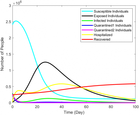
Figure 2. Simulation results in an endemic situation
Figure 2 shows an endemic situation where susceptible individuals decrease due to transmission from exposed and infected individuals, resulting in an increase in exposed individuals until the 27th day.
However, until the 10th day the quarantined-1 individual decreased, this was due to the quarantined-1 individual being able to recover to a suspectible individual. Likewise, quarantined-2 decreased until the 10th day because some of the quarantined-2 individuals were hospitalized and some death, either natural death or death coused by COVID-19 infected. On the 27th day, the exposed individuals reached the peak where the number reached more than 1.25×10⁶ individuals and after that it decreased, but for the infected individuals, it increased to a peak on the 29th day with the number of 0.13×10⁶ individuals and after that it decreased slowly. The increase in infected individuals was due to the addition of susceptible individuals infected with COVID-19.
Individuals treated by the medical team (hospitalized) increased and reached a peak on the 40th day where the number reached 0.584×10⁶ individuals, this was due to the addition of infected individuals and quarantine-2 to the hospitalized class. The increase in recovered individuals was due to individuals who were hospitalized some have recovered.
Figure 3. The effect of variations in parameter values q1 on the infected individuals
Further, simulated the effect of parameter variations q1 and q2 (parameter relating to quarantine) on infected individuals and reproductive number. Quarantine can be used as one of the mitigations to reduce the number of people infected with COVID-19 so that the COVID-19 disease does not spread. Quarantined simulation results are given in the Figure 3 and Figure 4 as follows.
The effect of the variation of parameter values q1 with other parameters remains constant, taking q1=0.085; and q1=0.383 and q1=0.993 changing the number of infected individuals is given in Figure 3.
It can be seen that the higher the parameter value q1 then the fewer infected individuals and vice versa. Until the 14th day with q1=0.085 people the number of infected individuals 26 730 people. While for, q1=0.383 infected individuals as many as 2,322 people. As q1=0.993 for the infected individuals as many as 8,250 people.
The effect of variations in parameter values q2 with other parameters remains constant, taking q2=0.085; and q2=0.383 and q2=0.993 on changes in the number of infected individuals is given in Figure 4.
Figure 4. The effect of variations in parameter values q1 on the Infected people
It can be seen that the higher the parameter value q2, so the fewer infected individuals and vice versa. Up to day 14th with q2=0.085 the number of infected individuals 43,710 people, for q2=0.383 those infected individuals as many as 25,070 people. As for q2=0.993 the infected individuals as many as 12,290 people. To investigate the quarantine effect, we took q1=0.5 and q2=0.4, while the other parameters were constant $R_0=0.2205$ and the non-endemic equilibrium point, $K^0=$ $\left (1.2909 \times 10^9; 0 ; 0 ; 0 ; 0\right)$. Since $R_0=0.2205<1$, this results in an asymptotically stable for non-endemic equilibrium point.
Figure 5. The effect of quarantine on the spread of COVID-19
This situation is given in Figure 5. It shows that if the parameter related to the quarantine can be maintained then the number of infected individuals will follow the curve according to the simulation results. In other words, the number of infected individuals will decrease over time. It means that the increasing value of the quarantine rate of exposed and infected individuals results in a smaller reproduction number due to quarantined individuals cannot transmit COVID-19 to other individuals.
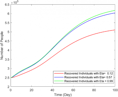
Figure 6. The effect of variations in parameter η on the Recovered people
The effect of parameter values η (transition rate from quarantined and infected individuals to hospitalized individuals) with other parameters remains constant, taking η=0.12; η=0.57; η=0.99 on changes in the number of recovered individuals is demonstrated in Figure 6.
It shown that the higher the parameter value $\eta$ then the higher recovered individuals. This is in accordance with the goals of hospitalized individuals for the treatment of infected individuals and accelerating recovery. Until the 14th day with η=0.12 people the number of recovered individuals 276,300 people. While for η=0.57, recovered individuals as many as 295,700 people. As η=0.99 for the recovered individuals as many as 298,500 people.
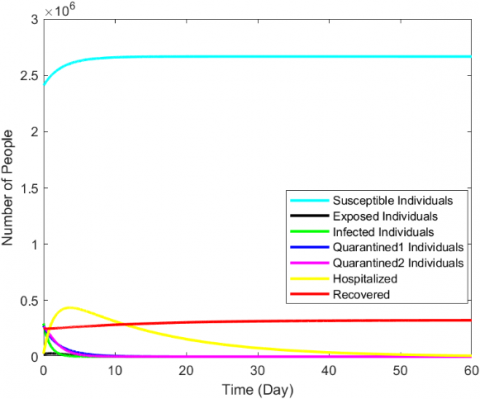
Furthermore, to investigate the quarantine and hospitalize effect, we took $q_1=0.5, q_2=0.4$ and $\eta=0.65$, while the other parameters were constant. The effect of quarantine and hospitalize on the dynamical model behaviour is depicted in Figure 7. This figure shows non endemic situation where susceptible individuals increase until the 18th day, which achieve 2,663,000 people. Meanwhile, on the 1st day, the number of exposed individual was 30,910 people and then decreased until 32nd day, which became 5 people. Likewise for the infected individuals on 3rd day, there were as many as 33,300 people, then it decreased until 40th day reached to 1 individual. It is also can be seen that for quarantine-1 and quarantine-2 individuals, on 4th day, there were as many as 66,620 and 101,400 people respectively, then it decreased to zero on 46th day. Meanwhile, individuals who were in the hospital on the 5th day were 373,400 people then decreased to 31,180 people on the 40th day, so there was a reduction of 342,220 people.
In addition, from Figure 7 it can be seen that recovered individuals increase over time, this is due to the intervention of quarantine and hospitalized individuals.
In this case, the basic reproduction value is $R_0=0.2192$. Since R0=0.2192<1, this results in an asymptotically stable for non-endemic equilibrium point. The reproduction number value with quarantine and hospitalized intervention is smaller than the reproduction number value with only quarantine intervention. This indicates that if quarantine and hospitalized are applied, than the COVID-19 disease in the future will disappear faster.
Figure 7. The effect of quarantine and hospitalize on the spread of COVID-19
We proposed in Section 2 the mathematical model that represents the dynamics of population in dealing with COVID-19 spread including a case study using data in Central Java Province, Indonesia presented in Section 5. In the case study we demonstrated a numerical simulation based on data variables (S,E,I,Q1,Q2,H,R) Central Java Province, Indonesia from 02 April 2021 to 5 October 2021 (about six months) to estimate the parameters. One may wonder whether these six-month data are sufficient. In fact, six months of data collection are enough because COVID-19 spread is not related to the annual cycle. For one year data, it does not significantly affect the transmission pattern of COVID-19 compared with six-month data. Besides, the analysis regarding the mathematical proofs and stability were completely observed in this study. For comparison purposes, some other published references also used data with less than or equal to six months of the observation in their models and have produced good simulation results (see e.g. [2, 4, 5, 11, 13, 15, 22, 24-26, 28]).
Numerical simulation results showed that the model has an endemic equilibrium point. In early stages, the number of individuals exposed and infected with COVID-19 increased, this is shown by the basic reproductive number value of 2.15, which means that one infected person can on average transmit the COVID-19 to two susceptible people. To reduce the reproduction number value, it can be done by increasing the average rate of exposed and infected individuals by applying self-quarantine and increasing the transition rate from quarantined and infected individuals to hospitalized individuals. This means that the more individuals who are quarantined, the number of infected individuals can be significantly reduced. Likewise, the more infected individuals who are admitted to the hospital, the faster the recovery. From the simulation results, by increasing quarantine and hospitalization, we found R0=0.2192<1. This condition results in an asymptotically stable non-endemic equilibrium point. This indicates that the transmission of COVID-19 is decreasing.
Based on the formulated model (1) this study still leaves open problems for future research prospects related to how to control the spread of COVID 19. Control variables could be added in the model that plays as strategies to reduce the number of exposed individual, quarantine individual, and infected individuals in the population and to increase the number of recovered individuals. Control variables could involve number of vaccinated individuals, self-precaution (wearing medical masks, washing hands/using hand sanitizers and physical distancing) and treatment. Furthermore, control methods that suit the dynamical model could be implemented in calculating the optimal strategy in controlling the spread of COVID-19. This will indeed produce more complicated differential equations and therefore further analysis regarding the existence and uniqueness of the optimal control are needed.
A modification of the SEIR dynamics model has been proposed by adding quarantine (Q) and hospitalized (H) variables to obtain the SEQ1Q2IHR dynamics model of the spread of COVID-19. In this case the population is divided into seven subpopulations, namely susceptible class, exposed, exposed individuals who were quarantined, infected individuals who were quarantined, infected, individuals being treated in hospital, and recovered. The dynamic model of the spread of COVID-19 has two equilibrium points, namely non-endemic and endemic.
We provided the conditions for the local stability of the non-endemic equilibrium point by using the Routh-Hurwith method and the global stability of the endemic equilibrium point which was investigated by using the Lyapunov method. It has been demonstrated that the non-endemic equilibrium point is locally asymptotically stable if the value of the basic reproduction number is less than one. The globally asymptotically stable endemic equilibrium point is achieved if the value of the basic reproduction number is more than one.
Furthermore, numerical simulations were carried out to verify the proposed model. Several scenarious were tested with various values of parameters related to quarantine and hospitalization. A relation between these parameters and the basic reproduction number was given, which showed that the increasing quarantine rate and hospitalization rate parameters resulted in a decreasing reproduction number. This means that the quarantine and hospitalization interventions can reduce the spread of the COVID-19 disease.
This work is supported by Diponegoro University, Indonesia, under RPI Research Grant with contract number 225-26/UN7.6.1/PP/2022. This research was supported by the Laboratory of Computer Modelling Mathematics Department, Faculty of Science and Mathematics, Diponegoro University, Semarang, Indonesia.
|
S |
Number of susceptible individuals |
|
E |
Number of exposed individuals |
|
I |
Number of infected individuals |
|
Q1 |
Number of exposed individuals who were quarantined |
|
Q2 |
Number of infected individuals who were quarantined |
|
H |
Number of hospitalized individua |
|
R |
Number of recovered individuals |
|
Greek Symbol |
|
|
A |
Rate of recruitment-S |
|
β1 |
Transmission rate in S from infected individual |
|
β2 |
Transmission rate in S from exposed individual |
|
μ1 |
Natural death rate |
|
μ2 |
Death rate caused by COVID-19 |
|
Ε |
Rate of development from Q1 to S |
|
q1 |
Rate of quarantine of exposed individuals |
|
q2 |
Rate of quarantine of infected individuals |
|
v |
Transition rate from Q1 to Q2 and E of I |
|
η |
Transition rate from Q2 and I to H |
|
γ |
Recovery rate of H |
Appendix A. Proof of Theorem 1
We know the initial conditions of $S(0) \geq 0, E(0) \geq$ $0, I(0) \geq 0, Q_1(0) \geq 0, Q_2(0) \geq 0, H(0) \geq 0 \quad$ and $R(0) \geq 0$, it will be shown that the solution $S(t)>0, E(t)>$ $0, I(t)>0, Q_1(t)>0, Q_2(t)>0, H(t)>0$ and $R(t)>$ 0for each $t>0$.
Consider the differential equation for the change in the number of susceptible individuals:
$\frac{d S}{d t}=A+\varepsilon Q_1-\beta_1 S I-\beta_2 S E-\mu_1 S$
$\frac{d S}{d t}=A+\varepsilon Q_1-\left(\beta_1 I+\beta_2 E+\mu_1\right) S$.
We can write the above equation as follows:
$\frac{d S(t)}{d t}+p S(t)=A+\varepsilon Q_1(t)$ where $p=\beta_1 I-\beta_2 E-\mu_1$
by using the integrating factor method, we can get:
$\frac{d S(t)}{d t} \cdot e^{\int_0^t p d \theta}+p S(t) \cdot e^{\int_0^t p d \theta}=\left(A+\varepsilon \cdot Q_1(t)\right) e^{\int_0^t p d \theta}\Leftrightarrow \frac{d}{d t}\left(S(t) \cdot e^{\int_0^t p d \theta}\right)=\left(A+\varepsilon \cdot Q_1(t)\right) e^{\int_0^t p d \theta}$
Furthermore, we find:
$\begin{aligned} S(t) \cdot e^{\int_0^t p d \theta}-S(0)= & \int_0^t\left(A+\varepsilon Q_1(t)\right) e^{\int_0^t p d \theta} d t S(t)= \\ S(0) e^{-\int_0^t p d \theta}+e^{-\int_0^t p d \theta} & \left\{\int_0^t\left(A+\varepsilon Q_1(t)\right) e^{\int_0^t p d \theta} d t\right\}>0 \forall t>0\end{aligned}$
In the same way, it can be obtained that $E(t)>0, I(t)>$ $0, Q_1(t)>0, Q_2(t)>0, H(t)>0$, and $R(t)>0$. Then the solution of $S(t), E(t), I(t), Q_1(t), Q_2(t), H(t)$, and $R(t)$ of the dynamic model (1) are positive for every $t>0$.
Appendix B. Proof of Theorem 2
Given $\quad N(t)=S(t)+E(t)+I(t)+Q_1(t)+Q_2(t)+$ $H(t)+R(t)$
$\frac{d N}{d t}=\frac{d S}{d t}+\frac{d E}{d t}+\frac{d I}{d t}+\frac{d Q_1}{d t}+\frac{d Q_2}{d t}+\frac{d H}{d t}+\frac{d R}{d t}$
$\frac{d N}{d t}=\left(A+\varepsilon Q_1-\beta S I-\beta \sigma S E-\mu_1 S\right)$
$+\left(\beta S I+\beta \sigma S E-q_1 E-\mu_1 E-v E\right)$
$+\left(v E-q_2 I-\eta I-\left(\mu_1+\mu_2\right) I\right)$
$+\left(q_1 E-\varepsilon Q_1-v Q_1-\mu_1 Q_1\right)$
$+\left(q_2 I+v Q_1-\eta Q_2-\left(\mu_1+\mu_2\right) Q_2\right)$
$+\left(\eta I+\eta Q_2-\gamma H-\left(\mu_1+\mu_2\right) H\right)+(\gamma H-\mu R)$
$\begin{aligned} \frac{d N}{d t} & =A+\varepsilon Q_1-\beta S I-\beta \sigma S E-\mu_1 S+\beta S I+\beta \sigma S E-q_1 E-\mu_1 E-v E \\ & +v E-q_2 I-\eta I-\mu_1 I-\mu_2 I+q_1 E-\varepsilon Q_1-v Q_1-\mu_1 Q_1+q_2 I+v Q_1 \\ & -\eta Q_2-\mu_1 Q_2-\mu_2 Q_2+\eta I+\eta Q_2-\gamma H-\mu_1 H-\mu_2 H-\mu_1 R\end{aligned}$
$\begin{aligned} \frac{d N}{d t}=A-\mu_1 S- & \mu_1 E-\mu_1 I-\mu_2 I-\mu_1 Q_1-\mu_1 Q_2-\mu_2 Q_2 \\ & -\mu_1 H-\mu_2 H-\mu_1 R \\ \frac{d N}{d t} \leq A-\mu_1 S- & \mu_1 E-\mu_1 I-\mu_1 Q_1-\mu_1 Q_2-\mu_1 H- \\ & \mu_1 R \frac{d N}{d t} \leq A-\mu_1 N\end{aligned}$.
An initial value N(0) that represents the total population at time t=0.
$\frac{d N(t)}{d t} e^{\int_0^t \mu_1 d y}+\mu_1 N(t) e^{\int_0^t \mu_1 d y} \leq A e^{\int_0^t \mu_1 d y}$
$\frac{d}{d t}\left(N(t) e^{\int_0^t \mu_1 d y}\right) \leq A e^{\int_0^t \mu_1 d y}$
$d\left(N(t) e^{\mu_1 t}\right) \leq A e^{\mu_1 t} d t$
$N(t) e^{\mu_1 t}-N(0) \leq \frac{A}{\mu_1}\left(e^{\mu_1 t}-1\right)$
$N(t) e^{\mu_1 t}-N(0) \leq \int_0^t A e^{\mu_1 t} d t$
For $t \rightarrow \infty$, we get $N(t) \leq \frac{A}{\mu_1}$
Then, all feasible solutions of model (1) are in the region $\Omega=\left\{\left(S(t), E(t), I(t), Q_1(t), Q_2(t), H(t), R(t)\right) \in \mathbb{R}_{+}^7: 0 \leq\right.$ $\left.N(t) \leq \frac{A}{\mu_1}\right\}$. Therefore, all solutions of system (1) are bounded.
Appendix C. Proof of Theorem 3
In carrying out a local stability analysis at the non-endemic equilibrium point (K0) of non-linear model (1) with linearization around K0.
As we know that the first five equation of the model (1) do not depend on H and R, so the system (1) can be reduced to a system with five variables $S, E, I, Q_1, Q_2$. Linearization of the system around non-endemic equilibrium point, we obtain Jacobian matrix $J\left(K^0\right)$ as follows
$\left(K^0\right)=\left[\begin{array}{ccccc}-\beta_1 I^0-\beta_2 E^0-\mu_1 & -\beta_2 S^0 & -\beta_1 S^0 & \varepsilon & 0 \\ \beta_1 I^0+\beta_2 E^0 & \beta_2 S^0-q_1-\mu_1-v & \beta_1 S^0 & 0 & 0 \\ 0 & v & -q_2-\eta-\left(\mu_1+\mu_2\right) & 0 & 0 \\ 0 & q_1 & 0 & -\varepsilon-v-\mu_1 & 0 \\ 0 & 0 & q_2 & v & -\eta-\left(\mu_1+\mu_2\right)\end{array}\right]$.
Base on Routh-Hurwith criterion, non-endemic equilibrium point K0 is locally asymptotically stable if the all eigenvalues of the Jacobian matrix have negative real parts. By calculating $\operatorname{det}\left(\lambda I-J\left(K^0\right)\right)=0$, where λ is the eigenvalues of the matrix $J\left(K^0\right)$, then the characteristic polinimial is obtained as follows.
$\left(\lambda+\mu_1\right)\left(\lambda+\varepsilon+v+\mu_1\right)\left(\lambda-\eta+\mu_1+\mu_2\right)\left(\lambda+q_2+\eta+\right.\left.\mu_1+\mu_2\right)\left(\lambda-\frac{\beta_2 A-\mu_1^2-q_1 \mu_1-v \mu_1}{\mu_1}\right)=0,$
which means the eigenvalues are as follows
$\lambda_1=-\mu_1 \quad \lambda_4=-q_2-\eta-\mu_1-\mu_2$
$\begin{aligned} & \lambda_2=-\varepsilon-v-\mu_1 \\ & \lambda_3=\eta-\mu_1-\mu_2\end{aligned} \quad \lambda_5=\frac{\beta_2 A-\mu_1^2-q_1 \mu_1-v \mu_1}{\mu_1}$.
Note that the matrix $J\left(K^0\right)$ has three strictly negative eigenvalues $\left(\lambda_1, \lambda_2, \lambda_4\right)$. The eigenvalues of $\lambda_3$ and $\lambda_5$ are negative if $\eta<\mu_1+\mu_2$ and $\beta_2 A<\mu_1^2+q_1 \mu_1+v \mu_1$. Since three negative eigenvalues and two conditionally negative eigenvalues are obtained from the Jacobian matrix $J\left(K^0\right)$, it's indicate that the non-endemic equilibrium point is locally asymptotically stable for $\mathfrak{R}_0$ less than one.
[1] Arin, J., Portet, S. (2021). A simple model for COVID-19. Infect. Dis. Model, 5: 309-315. https://doi.org/10.1016/j.idm.2020.04.002
[2] Roberto Telles, C., Lopes, H., Franco, D. (2021). SARS-COV-2: SIR model limitations and predictive constraints. Symmetry, 13(4): 676. https://doi.org/10.3390/sym13040676
[3] Frausto-Solís, J., Hernández-González, L.J., González-Barbosa, J.J., Sánchez-Hernández, J.P., Román-Rangel, E. (2021). Convolutional neural Network–Component transformation (CNN–CT) for confirmed COVID-19 cases. Mathematical and Computational Applications, 26(2): 29. https://doi.org/10.3390/mca26020029
[4] Wu, K., Darcet, D., Wang, Q., Sornette, D. (2020). Generalized logistic growth modeling of the COVID-19 outbreak: Comparing the dynamics in the 29 provinces in China and in the rest of the world. Nonlinear dynamics, 101(3): 1561-1581. https://doi.org/10.1007/s11071-020-05862-6
[5] Zhao, S., Lin, Q., Ran, J., Musa, S.S., Yang, G., Wang, W., Wang, M.H. (2020). Preliminary estimation of the basic reproduction number of novel coronavirus (2019-nCoV) in China, from 2019 to 2020: A data-driven analysis in the early phase of the outbreak. International Journal of Infectious Diseases, 92: 214-217. https://doi.org/10.1016/j.ijid.2020.01.050
[6] Ahmed, M.I.B., Rahman, A.U., Farooqui, M., Alamoudi, F., Baageel, R., Alqarni, A. (2021). Early identification of COVID-19 using dynamic fuzzy rule based system. Mathematical Modelling of Engineering Problems, 8(5): 805-812. https://doi.org/10.18280/mmep.080517
[7] Mishra, B.K., Keshri, A.K., Rao, Y.S., Mishra, B.K., Mahato, B., Ayesha, S., Singh, A.K. (2020). COVID-19 created chaos across the globe: Three novel quarantine epidemic models. Chaos, Solitons & Fractals, 138: 109928. https://doi.org/10.1016/j.chaos.2020.109928
[8] Okafor, S.O., Ugwu, C.I., Nkwede, J.O., Onah, S., Amadi, G., Udenze, C., Chuke, N. (2022). COVID-19 public health and social measures in Southeast Nigeria and its implication to public health management and sustainability. Opportunities and Challenges in Sustainability, 1(1): 61-75. https://doi.org/10.56578/ocs010107
[9] Widowati, Sutimin. (2013). Pemodelan Matematika, Analisis dan Aplikasinya. Semarang: Undip Press Semarang.
[10] Deng, X., Kong, Z. (2021). Humanitarian rescue scheme selection under the COVID-19 crisis in China: Based on group decision-making method. Symmetry, 13(4): 668. https://doi.org/10.3390/sym13040668
[11] Ala’raj, M., Majdalawieh, M., Nizamuddin, N. (2021). Modeling and forecasting of COVID-19 using a hybrid dynamic model based on SEIRD with ARIMA corrections. Infectious Disease Modelling, 6: 98-111. https://doi.org/10.1016/j.idm.2020.11.007
[12] Adedotun, A.F. (2022). Hybrid neural network prediction for time series analysis of COVID-19 cases in Nigeria. Journal of Intelligent Management Decision, 1(1): 46-55. https://doi.org/10.56578/jimd010106
[13] Mackolil, J., Mahanthesh, B. (2020). Logistic growth and SIR modelling of Coronavirus disease (COVID-19) outbreak in India: Models based on real-time data. Mathematical Modelling of Engineering Problems, 7(3): 345-350. https://doi.org/10.18280/mmep.07030
[14] ud Din, R., Seadawy, A.R., Shah, K., Ullah, A., Baleanu, D. (2020). Study of global dynamics of COVID-19 via a new mathematical model. Results in Physics, 19: 103468. https://doi.org/10.1016/j.rinp.2020.103468
[15] Carcione, J.M., Santos, J.E., Bagaini, C., Ba, J. (2020). A simulation of a COVID-19 epidemic based on a deterministic SEIR model. Frontiers in Public Health, 8: 230. https://doi.org/10.3389/fpubh.2020.00230
[16] Santoro, A., López Osornio, A., Williams, I., Wachs, M., Cejas, C., Havela, M., Rubinstein, A. (2022). Development and application of a dynamic transmission model of health systems’ preparedness and response to COVID-19 in twenty-six Latin American and Caribbean countries. PLOS Global Public Health, 2(3): e0000186. https://doi.org/10.1371/journal. pgph.0000186
[17] Parsamanesh, M., Erfanian, M., Mehrshad, S. (2020). Stability and bifurcations in a discrete-time epidemic model with vaccination and vital dynamics. BMC Bioinformatics, 21(1): 1-15. https://doi.org/10.1186/s12859-020-03839-1
[18] Tchoumi, S.Y., Rwezaura, H., Tchuenche, J.M. (2022). Dynamic of a two-strain COVID-19 model with vaccination. Results in Physics, 39: 105777. https://doi.org/10.1016/j.rinp.2022.105777
[19] Rahman, B., Khoshnaw, S.H., Agaba, G.O., Al Basir, F. (2021). How containment can effectively suppress the outbreak of COVID-19: A mathematical modeling. Axioms, 10(3): 204. https://doi.org/10.3390/axioms10030204
[20] Masoumnezhad, M., Rajabi, M., Chapnevis, A., Dorofeev, A., Shateyi, S., Kargar, N.S., Nik, H.S. (2020). An approach for the global stability of mathematical model of an infectious disease. Symmetry, 12(11): 1778. https://doi.org/10.3390/sym12111778
[21] Radha, M., Balamuralitharan, S. (2020). A study on COVID-19 transmission dynamics: stability analysis of SEIR model with Hopf bifurcation for effect of time delay. Advances in Difference Equations, 2020(1): 1-20. https://doi.org/10.1186/s13662-020-02958-6
[22] Serhani, M., Labbardi, H. (2021). Mathematical modeling of COVID-19 spreading with asymptomatic infected and interacting peoples. Journal of Applied Mathematics and Computing, 66(1): 1-20. https://doi.org/10.1007/s12190-020-01421-9
[23] Sugiyanto, S., Abrori, M. (2020). A mathematical model of the Covid-19 Cases in Indonesia (under and without lockdown enforcement). Biology, Medicine, & Natural Product Chemistry, 9(1): 15-19. https://doi.org/10.14421/biomedich.2020.91.15-19
[24] Manna, S., Chowdhury, T., Dhar, A.K., Nieto, J.J. (2021). On mathematical modelling of the Indian human hair industry in the Post-COVID-19 era. Mathematical Modelling of Engineering Problems, 8(3): 447-452. https://doi.org/10.18280/mmep.080315
[25] Hu, Z., Cui, Q., Han, J., Wang, X., Wei, E.I., Teng, Z. (2020). Evaluation and prediction of the COVID-19 variations at different input population and quarantine strategies, a case study in Guangdong province, China. International Journal of Infectious Diseases, 95: 231-240. https://doi.org/10.1016/j.ijid.2020.04.010
[26] Cullenbine, C.A., Rohrer, J.W., Almand, E.A., Steel, J.J., Davis, M.T., Carson, C.M., Wickert, D.P. (2021). Fizzle testing: an equation utilizing random surveillance to help reduce COVID-19 risks. Mathematical and Computational Applications, 26(1): 16. https://doi.org/10.3390/mca26010016
[27] Bärwolff, G. (2020). Mathematical modeling and simulation of the COVID-19 pandemic. Systems, 8(3): 24. https://doi.org/10.3390/systems8030024
[28] Zewdie, A.D., Gakkhar, S. (2020). A Mathematical Model for Nipah Virus Infection. Journal of Applied Mathematics, 2020: Article ID 6050834. https://doi.org/10.1155/2020/6050834
[29] Yang, C., Wang, J. (2020). A mathematical model for the novel coronavirus epidemic in Wuhan, China. Mathematical Biosciences and Engineering: MBE, 17(3): 2708-2724. https://doi.org/10.3934/mbe.2020148
[30] Ishtiaq, A. (2020). Dynamics of COVID-19 transmission: compartmental-based mathematical modeling. Life and Science, 1(Suppl): 128-132. http://doi.org/10.37185/LnS.1.1.134
[31] Schecter, S. (2021). Geometric singular perturbation theory analysis of an epidemic model with spontaneous human behavioral change. Journal of Mathematical Biology, 82(6): 1-26. https://doi.org/10.1007/s00285-021-01605-2
[32] Lamichhane, S., Chen, Y. (2015). Global asymptotic stability of a compartmental model for a pandemic. Journal of the Egyptian Mathematical Society, 23(2): 251-255. http://dx.doi.org/10.1016/j.joems.2014.04.001