Waleed Altalabani* | Yaser Alaiwi
© 2022 IIETA. This article is published by IIETA and is licensed under the CC BY 4.0 license (http://creativecommons.org/licenses/by/4.0/).
OPEN ACCESS
Quadcopters have unstable systems, and one of the main reasons for the irregularity of their systems may be the behavior of the output of certain types of control units. But the development that an event in the control methods made the control of these systems very effective to achieve the maximum stability required. Examples of methods with modern controllers we mention here are the linear quadratic regulator (LQR) controller, Besides the (MPC) model predictive controller, there is also the integral proportionally derivative (PID)which we worked on developing in this research. This paper aims to deal with compensation for position tracking error of quadrotor. To address this problem, we designed an adaptive PID controller that enhances the tracking performance and tests the proposed controller on two different trajectories against the performance of the normal PID controller. Through the simulation results using MATLAB the suggested strategy was shown to be effective in lowering the errors associated tracking of intended trajectories in X and Y orientations.
adaptive, PID controller, unmanned aerial vehicle, quadrotor
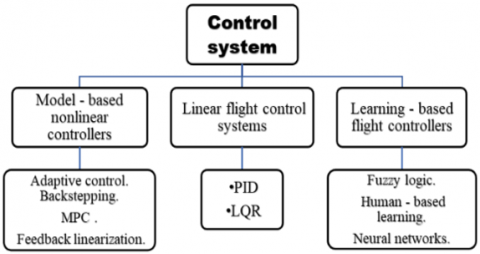
The operation of control systems has been extensively discussed in the literature during the last two decades. and how they can be used to control drones. This has led to the development of different techniques and methods. In each category the high-level methods are grouped according to the algorithmic approach used, which in most cases is related to used type of sensors. Main control techniques can be categorized as follows:
This category includes several control methods but the most commonly used are the ones based on, neural networks, human-based learning, and fuzzy logic.
Here we highlight an important approach in this denomination is proportionally integral derivative (PID) and best-known and most extensively utilized control in this area; another widely used method is the linear quadratic regulator (LQR) controller.
Adaptive control tops the methods in this category, while backstepping, model predictive control MPC and feedback linearization are examples of other commonly used ones.
Figure 1 bellow shows categorization of control techniques.
Most of these methods are not used alone, usually two or even three methods are integrated together to achieve optimal control of the drone. In the following lines we review several research studies for different control methods.
A backstepping-based direct-dynamic adaptive controller was provided to follow the trajectory of a quadcopter, while ensuring global stability using Lyapunov's theory. The proposed method has proven feasibility and acceptable convergence results [1]. Precise model parameters are required for any algorithm based on general backstepping control; this control doesn’t perform well when there are external disturbances. To solve this problem, a control algorithm based on adaptive integral backstepping was developed. The results obtained after simulation demonstrated that the developed control performs well against model uncertainties [2]. A powerful control technique was introduced using adaptive neural control to stabilize and track the quadcopter when it is assumed that the aerodynamic drag coefficient is unknown. Numerical simulation demonstrates the efficiency of the introduced control approach [3].
Figure 1. Categorization of control techniques
The strategic way to control a quadcopter is based on active fault tolerance and focuses on Gain-Scheduled PID control was presented. Effectiveness of the introduced control method was proven by simulation [4]. The position tracking error of a quadcopter was compensated by an adaptive controller that aims to compensate the constant or slow-changing disturbance which represents wind and drafts, the system was able to reduces tracking error and is feasible for practical quadrotor use [5].
An SMC-based controller was developed for quadcopters to help with stability and altitude tracking, numerical simulations show the robustness of the introduced method [6]. A new nonlinear approach for adaptive control based on robust fixed-point was presented to provide remedy to parameters uncertainties or outer disturbances. Controller efficiency was demonstrated by simulation with multiple trajectories [7]. A controller based on improved adaptive SMC was introduced aiming to deal with navigation and control of a quadcopter when uncertainty and external disturbances existed. The obtained results proved the scheme’s robustness in the presence of uncertainties and effectiveness in tracking trajectories [8].
The controlling of the quadrotor was proposed using an adaptive controller that doesn’t require any information on model parameters. The results show effectiveness of the system and corroborated the analysis [9]. To control a quadcopter a new controller based on emotional learning was proposed a novel bidirectional algorithm for emotional learning is used in conjunction with an easier fuzzy neural network within the confines of this feature technique, the outcomes showed that the suggested approach performed admirably, as shown by the findings [10]. While in reference [11], sliding mode control using neural network backpropagation using three alternative paths and numerous circumstances with and without external disturbances was examined. Simulated results using MATLAB prove the SMC-NN control system's tracking performance and capacity to reach the target trajectory in the face of external disturbances.
Trajectory tracking of a quadcopter using self-tuning PD-fuzzy controller was introduced, the simulation proved the usefulness of the system for a fixed -gain aircraft as well as a control algorithm [12].
Gain scheduling SMC controller for quadrotor based on adaptive fuzzy was proposed to minimize the chattering of the conventional SMC, the results show a significant improvement in terms of reduced chattering with improved trajectory tracking [13]. An adaptive controller that combines a PID controller and According to the findings, the FPID controller outperforms the standard PID controller when the wind is blowing [14]. An adaptive controller for a quadrotor based on Lyapunov stability was introduced, the simulation demonstrated that the system provides greater benefits over the fixed-gain approach [15]. A quadcopter tracking control based on adaptive controller was presented, it enables the controller to follow the programmed path without knowing the inertia and was able reduce tracking errors when unstructured disturbances occur [16]. A decentralized adaptive control scheme was introduced to control a quadrotor, the system combines PD controller and auxiliary term with variable coefficient. The efficiency and robustness of the controller was demonstrated by simulation results [17]. Quadrotor trajectory tracking was achieved using An L1 adaptive controller based on nonlinear feedforward compensation, the simulation validated the efficiency of the introduced method [18].
A quadcopter controller which combines fuzzy logic and neural network was proposed tracking a quadrotor's trajectory, The data shows the system’s ability to follow a quadrotor’s trajectory [19]. An adaptive quadcopter path tracking controller was developed. The findings showed that the quadrotor control system is capable of producing smooth and continuous motions [20]. To enhance path tracking of quadrotor, an adaptive controller based on backstepping approach was proposed, the simulation results show robustness and applicability of the system [21].
In the design and implementation of a NARMA-L2 IFC-based intelligent control method for nonlinear dynamical systems. Through simulation results, the accuracy of control performance and the resilience of the proposed control mentioned above against external disturbances are proven for nonlinear plants [22].
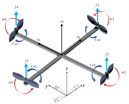
The quadrotor consists of four propellers in “X” configuration, these propellers are divided into two pairs (1, 3) and (2, 4) both sets of propellers are rotating counterclockwise, and this is to adjust the reactive torque effect by compensating, which has an important effect.
A quadcopter moves vertically by adjusting the speed of its four propellers; pitches as well as rolls by varying the speed of the front and rear propellers or left and right propellers; and yaw by varying the reactive torque of its four fans.
Figure 2. Physical illustration of a quadcopter
According to the Figure 2, the quadcopter kinematics is described by $x, y$, and $z$ in the $\mathrm{E}-$ framework (earth or ground inertial frame) and the B-frame (body-fixed framework) by $B=$ $\left(\mathrm{x}_{\mathrm{B}}, \mathrm{y}_{\mathrm{B}}, \mathrm{z}_{\mathrm{B}}\right)$. It is possible to calculate where the quadcopter's center of mass is in relation to E-frame $x, y, z$ axis with $\Gamma$. We can also determine the angular position in $\mathrm{E}$-frame with three Euler angles $\Phi$ as shown in Eq. (1). There's also a yaw angle $\psi$, a pitch angle $\theta$, and $\varphi$ an angle of roll.
$\Gamma^E=\left[\begin{array}{c}x^E \\ y^E \\ z^E\end{array}\right], \Phi^E=\left[\begin{array}{c}\varphi \\ \theta \\ \psi\end{array}\right]$ (1)
$V^B$ and $\omega^B$ are the formulas for calculating linear and angular velocities, respectively.
$V^B=\left[\begin{array}{c}u \\ \mathrm{v} \\ \mathrm{W}\end{array}\right], \omega^B=\left[\begin{array}{l}p \\ q \\ \mathrm{r}\end{array}\right]$ (2)
Vector Ψ contains the linear and angular position vectors and it is obtained from combining Eqns. (1) and (2):
$\Psi^{\prime}=\left[\begin{array}{l}\Gamma \\ \Phi\end{array}\right]=\left[\begin{array}{c}x^E \\ y^E \\ z^E \\ \varphi \\ \theta \\ \psi\end{array}\right]$ (3)
Vector W contains the linear and angular velocities vectors and it is obtained from combining Eq. (2):
$\mathrm{W}=\left[\begin{array}{l}V^B \\ \omega^B\end{array}\right]=\left[\begin{array}{l}u \\ \mathrm{v} \\ \mathrm{w} \\ p \\ q \\ \mathrm{r}\end{array}\right]$ (4)
The following is the rotational matrix for linear velocity transfer from the (B to E) framework.
$R=\left[\begin{array}{ccc}\cos (\psi) \cos (\theta) & \cos (\psi) \sin e(\theta) \sin e(\varphi)-\sin (\psi) \cos (\varphi) & \cos (\psi) \sin e(\theta) \cos (\varphi)+\sin e(\psi) \sin e(\varphi) \\ \sin e(\psi) \cos (\theta) & \sin e(\psi) \sin e(\theta) \sin e(\varphi)+\cos (\psi) \cos (\varphi) & \sin e(\psi) \sin e(\theta) \cos (\varphi)-\cos (\psi) \sin e(\varphi) \\ -\sin e(\theta) & \cos (\theta) \sin e(\varphi) & \cos (\theta) \cos (\varphi)\end{array}\right]$ (5)
The turnover matrix $R$ is orthonormal where here $R^{-1}=R^T$, and this means that it is the rotation from (E to B)framework.
The matrix for changing angular speeds from (E to B)-framework is $W_{\Phi}$, and from (B to $\mathrm{E}$ )-framework is $W_{\Phi}{ }^{-1}$.
$\dot{\Phi}^E=\mathrm{W}_{\Phi}{ }^{-1} \omega^B,\left[\begin{array}{c}\dot{\varphi} \\ \dot{\theta} \\ \dot{\psi}\end{array}\right]$$=\left[\begin{array}{ccc}1 & \operatorname{sine}(\varphi) \tan (\theta) & \cos (\varphi) \tan (\theta) \\ 0 & \cos (\varphi) & -\operatorname{sine}(\varphi) \\ 0 & \frac{\sin e(\varphi)}{\cos (\theta)} & \frac{\cos (\varphi)}{\cos (\theta)}\end{array}\right]\left[\begin{array}{l}p \\ q \\ r\end{array}\right]$ (6)
Whereas $\dot{\Phi}^{\mathrm{E}}$ indicates the E-framework angular velocity regarding the B -framework.
As a possible consequence, the B-angular frame velocity is as:
$\omega^B=W_{\Phi} \dot{\Phi^E},\left[\begin{array}{l}p \\ q \\ r\end{array}\right]=\left[\begin{array}{ccc}1 & 0 & -\sin (\theta) \\ 0 & \cos (\varphi) & \cos (\theta) \sin (\varphi) \\ 0 & -\sin (\varphi) & \cos (\theta) \cos (\varphi)\end{array}\right]\left[\begin{array}{c}\dot{\varphi} \\ \dot{\theta} \\ \dot{\psi}\end{array}\right]$ (7)
$W_{\Phi}$ reversible if $\theta \neq \frac{(2 k-1) \varphi}{2},(k \in Z)$.
We presume that the quadcopter is symmetrical, and that each propeller has the same length of arm. By aligning the arms with the body’s x and y plane coordinates, slant inertia matrix is created because of symmetry, Ixx=Iyy.
$I=\left[\begin{array}{ccc}I_{x x} & 0 & 0 \\ 0 & I_{y y} & 0 \\ 0 & 0 & I_{z z}\end{array}\right]$ (8)
A thrust force perpendicular to B-frame is generated by the angular velocity of each propeller, there is a torque about the rotor axis is also generated. As given in Eqns. (9) and (10) as follows:
$\mathrm{f}_{\mathrm{i}}=k \mathrm{w}_{\mathrm{i}}^2$ (9)
$\tau_{\mathrm{M}_i}=b \mathrm{w}_{\mathrm{i}}^2+\mathrm{I}_{\mathrm{M}} \dot{\mathrm{W}}_1$ (10)
where, k is the constant for lift, b is the constant for drag, and $I_M$, the rotors inertial. In most cases, the impact angular acceleration wi is thought to be small, so it is left out. When we add up the forces of commonality of four propellers, we get the thrust T straight the body's airframe z-axis, as shown in Eq. (11).
$T=\sum_{i=1}^4 \mathrm{f}_{\mathrm{i}}=k \sum_{i=1}^4 \mathrm{w}_{\mathrm{i}}^2, T^B=\left[\begin{array}{l}0 \\ 0 \\ \mathrm{~T}\end{array}\right]$ (11)
By combining the torques of all four propellers we obtain the vector τB This represents the torques along each of the main body orientations $\left(\tau_{\varphi}, \tau_\theta\right.$ and $\left.\tau_\psi\right)$ as shown in Eq. (12):
$\tau_{\mathrm{B}}=\left[\begin{array}{l}\tau_{\varphi} \\ \tau_\theta \\ \tau_{\Psi}\end{array}\right]=\left[\begin{array}{c}l k\left(-\mathrm{w}_2^2+\mathrm{w}_4^2\right) \\ l k\left(-\mathrm{w}_1^2+\mathrm{w}_3^2\right) \\ k \sum_{i=1}^4 \tau_{\mathrm{M}_i}\end{array}\right]$ (12)
Whereas l a quadcopter's rotor-to-center-of-mass distance.
Since the quadrotor is rigid body, Newton -Euler formulas are used to explain its dynamics. For B-frame, the quantitative of acceleration force $m \dot{V}^B$ with centrifugal force $\omega^B \times m V^B$ are the same as the gravitational force $R^T G$ as well as the thrust produced by the propellers $T_B$.
$\dot{mV^B}+\omega^B \times m V^B=R^T G+T_B$ (13)
In Earthly-frame, the centrifugal- force is cancelled out, so the quadrotor's acceleration comes from gravity and the type and direction of all thrust:
$m \ddot{\Gamma}=G+R \mathrm{~T}_{\mathrm{B}}$ (14)
$\left[\begin{array}{c}\ddot{x} \\ \ddot{y} \\ \ddot{z}\end{array}\right]=-g\left[\begin{array}{l}0 \\ 0 \\ 1\end{array}\right]+\frac{T}{m}$$\left[\begin{array}{c}\cos (\psi) \sin e(\theta) \operatorname{sine}(\varphi)+\operatorname{sine}(\psi) \sin e(\varphi) \\ \sin e(\psi) \sin e(\theta) \cos (\varphi)-\cos (\psi) \sin e(\varphi) \\ \cos (\theta) \cos (\varphi)\end{array}\right]$ (15)
In the Body-frame, the inertia's angular acceleration $\dot{I{V}^B}$, centripetal forces $\omega^B \times I \omega^B$, and gyroscopic forces $\Theta$are all equivalent to the external torque τ.
$\dot{I{V}^B}+\omega^B \times I \omega^B+\Theta=\tau$ (16)
Then, the transformation matrix $\mathrm{W}_{\Phi}{ }^{-1}$ and its temporal derivative are used to get angular accelerations in the E-frame from accelerations in the B-frame:
$\ddot{\Phi}=\frac{d}{d t}\left(\mathrm{~W}_{\Phi}^{-1} \omega^B\right)=\frac{d}{d t}\left(\mathrm{~W}_{\Phi}^{-1}\right) \omega^B+\mathrm{W}_{\Phi}{ }^{-1} \dot{V^B}$
$=\left[\begin{array}{ccc}0 & \dot{\varphi} \cos (\varphi) \tan (\theta)+\dot{\theta} \frac{\sin e(\varphi)}{\cos (\theta)^2} & -\dot{\varphi} \operatorname{sine}(\varphi) \cos (\theta)+\dot{\theta} \frac{\cos (\varphi)}{\cos (\theta)^2} \\ 0 & -\dot{\varphi} \operatorname{sine}(\varphi) & -\dot{\varphi} \cos (\varphi) \\ 0 & \dot{\varphi} \frac{\cos (\varphi)}{\cos (\theta)}+\frac{\dot{\varphi} \sin e(\varphi) \tan (\theta)}{\cos (\theta)} & -\dot{\varphi} \frac{\sin e(\varphi)}{\cos (\theta)}+\frac{\dot{\varphi} \cos (\varphi) \tan (\theta)}{\cos (\theta)}\end{array}\right]$$\omega^B+\mathrm{W}_{\Phi}{ }^{-1} \dot{V^B}$ (17)
Rotational and translational energies subtract potential energy are equal to the total of LaGrange L.
$\mathcal{L}(\mathrm{q}, \dot{\mathrm{q}})=\mathrm{E}_{\text {trans }}+\mathrm{E}_{\mathrm{rot}}-\mathrm{E}_{\mathrm{pot}}=\left(\frac{\mathrm{m}}{2}\right) \dot{\Gamma}^T \dot{\Gamma}+\left(\frac{1}{2}\right) \omega^{B^T} I \omega^B=-m g z$ (18)
The Euler-Lagrange formulas with exterior forces and also torques are presented in Eq. (10).
$\left[\begin{array}{l}\mathrm{f} \\ \tau\end{array}\right]=\frac{d}{d t}\left(\frac{\partial \mathcal{L}}{\partial \dot{\mathrm{q}}}\right)-\frac{\partial \mathcal{L}}{\partial \mathrm{q}}$ (19)
We will study the linear and angular components separately since they are undependable. The total thrust of the rotors constitutes the linear external force. Formulas of a linear Euler-Lagrange format equation.
$\mathrm{f}=\mathrm{RT}_{\mathrm{B}}=m \ddot{\Gamma}+\mathrm{mg}\left[\begin{array}{l}0 \\ 0 \\ 1\end{array}\right]$ (20)
which corresponds to Eq. (18).
$\left\{\begin{array}{c}\ddot{x}=\frac{1}{m}(\cos (\varphi) \cos (\psi) \sin e(\theta)+\sin e(\varphi) \sin e(\psi)) u_1 \\ \ddot{y}=\frac{1}{m}(\cos (\varphi) \sin e(\psi) \sin e(\theta)-\sin e(\varphi) \cos (\psi)) u_1 \\ z=\frac{1}{m} \cos (\varphi) \cos (\theta) u_1-g\end{array}\right.$ (21)
This is the Jacobian matrices $J(\Phi)$ the regarding from $\omega^B$ to $\dot{\Phi}$ :
$\mathrm{J}(\Phi)=\mathrm{J}=\mathrm{w}_{\Phi}{ }^T I W_{\Phi}=$$\left[\begin{array}{ccc}\mathrm{I}_{\mathrm{xx}} & 0 & -\mathrm{I}_{\mathrm{xx}} \sin e(\theta) \\ 0 & \mathrm{I}_{\mathrm{yy}} \cos (\varphi)^2+\mathrm{I}_{\mathrm{zz}} \sin e(\varphi)^2 & \left(\mathrm{I}_{\mathrm{yy}}-\mathrm{I}_{\mathrm{zz}}\right) \cos (\varphi) \sin e(\varphi) \cos (\theta) \\ -\mathrm{I}_{\mathrm{xx}} \sin e(\theta) & \left(\mathrm{I}_{\mathrm{yy}}-\mathrm{I}_{\mathrm{zz}}\right) \cos (\varphi) \sin e(\varphi) \cos (\theta) & \mathrm{I}_{\mathrm{xx}} \sin e(\theta)^2+\mathrm{I}_{\mathrm{yy}} \operatorname{sine}(\varphi)^2 \cos (\theta)^2+\mathrm{I}_{\mathrm{zz}} \cos (\varphi)^2 \cos (\theta)^2\end{array}\right]$ (22)
Therefore, in the E-framework, rotational energy is as specified:
$\mathrm{E}_{\text {rot }}=\left(\frac{1}{2}\right)\left(\dot{\mathrm{V}}^{\mathrm{B}}\right)^T I \omega^B=(1 / 2) \ddot{\Phi}^T J \ddot{\Phi}$ (23)
The exterior angular force consists of all rotors torques. The angles are described by the Euler-Lagrange equations as follows:
$\tau=\tau_B=J \ddot{\Phi}+\frac{d}{d t}(J) \dot{\Phi}-\frac{1}{2} \frac{\partial}{\partial \eta}\left(\dot{\Phi}^T J \dot{\Phi}\right)$$=J \ddot{\Phi}+C(\Phi, \dot{\Phi}) \dot{\Phi}$ (24)
Below is a clear visualization of the gyroscope and gravity equations.
This is how the matrix $C(\Phi, \dot{\Phi})$ is written:
$C(\Phi, \dot{\Phi})\left[\begin{array}{lll}C_{11} & C_{12} & C_{13} \\ C_{21} & C_{22} & C_{23} \\ C_{31} & C_{32} & C_{33}\end{array}\right]$ (25)
We can obtain the differential equations from Eq. (26) for the angular accelerations:
$\ddot{\Phi}=\mathrm{J}^{-1}\left(\mathrm{\tau}_B-C(\Phi, \dot{\Phi}) \dot{\Phi}\right)$
$\ddot{\varphi}=\frac{\mathrm{I}_{\mathrm{y}}-\mathrm{I}_{\mathrm{z}}}{\mathrm{I}_{\mathrm{x}}} \dot{\theta} \dot{\psi}-\frac{\mathrm{I}_{\mathrm{r}}}{\mathrm{I}_{\mathrm{x}}} \Omega_{\mathrm{r}} \dot{\theta}+\frac{1}{\mathrm{I}_{\mathrm{x}}} \mathrm{u}_2$
$\ddot{\theta}=\frac{\mathrm{I}_{\mathrm{z}}-\mathrm{I}_{\mathrm{c}}}{\mathrm{I}_{\mathrm{y}}} \dot{\theta} \dot{\psi}-\frac{\mathrm{I}_{\mathrm{r}}}{\mathrm{I}_{\mathrm{y}}} \Omega_{\mathrm{r}} \dot{\varphi}+\frac{1}{\mathrm{I}_{\mathrm{y}}} \mathrm{u}_3$ (26)
$\ddot{\Psi}=\frac{\mathrm{I}_{\mathrm{x}}-\mathrm{I}_{\mathrm{y}}}{\mathrm{I}_{\mathrm{z}}} \dot{\theta} \dot{\varphi}+\frac{1}{\mathrm{I}_{\mathrm{z}}} \mathrm{u}_4$
From (25) and (26) we can find the equations of motion for translational and rotational movement of the quadcopter system.
We will use a simplified model because we will not take the influence of aerodynamical effects in consideration since it is very complicated and hard to model, and it effects only at high speeds.
5.1 PID control
Many linear and non-linear applications often employ PID controllers, which are very strong and helpful. The error signal e(t) is calculated as follows:
$e(t)=$ desired input $(t)-$ actual outpot $(t)$
By adjustment of a control variable u(t), The goal of the controller is to gradually reduce the number of mistakes. PID
$u(t)=\mathrm{k}_{\mathrm{p}} e(t)+\mathrm{k}_{\mathrm{i}} \int e(t)+\mathrm{k}_{\mathrm{d}} \frac{d}{d t} e(t)$ (27)
PID controller also calculates an error value e(t) on a continuous basis then applies the corrections depending on proportional, integral, and derivative terms.
5.2 Adaptive PID control
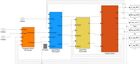
To extend our study and optimize the quadrotor control we design an adaptive controller that is integrated with the traditional PID controller. This adaptive controller is mainly. based on a Gaussian function that makes the error value e(t) varies and not constant. Figure 3 shows the integrated adaptive controller.
Figure 3. Quadrotor and controller Simulink model
5.3 Controller objective
For the purpose of controlling motor speed, a controller PID or adaptive PID are used, in a way that the quadrotor able to follow the desired trajectory. The control inputs can be demonstrated as:
$\left[\begin{array}{l}u_1 \\ u_2 \\ u_3 \\ u_4\end{array}\right]=\left[\begin{array}{c}F \\ \tau_\theta \\ \tau_{\varphi} \\ \tau_{\Psi}\end{array}\right]=\left[\begin{array}{cccc}b & b & b & b \\ 0 & -l b & 0 & l b \\ -l b & b & l b & 0 \\ d & -d & d & -d\end{array}\right]\left[\begin{array}{l}\omega_1^2 \\ \omega_2^2 \\ \omega_3^2 \\ \omega_4^2\end{array}\right]$ (28)
$\begin{aligned} \omega_1^2 & =\frac{u_1}{4 b}-\frac{u_3}{2 l b}+\frac{u_4}{4 d} \\ \omega_2^2 & =\frac{u_1}{4 b}-\frac{u_2}{2 l b}-\frac{u_4}{4 d} \\ \omega_3^2 & =\frac{u_1}{4 b}+\frac{u_3}{2 l b}+\frac{u_4}{4 d} \\ \omega_4^2 & =\frac{u_1}{4 b}+\frac{u_2}{2 l b}-\frac{u_4}{4 d}\end{aligned}$ (29)
The whole system, including the controller, is represented in Figure 4.
6.1 Rectangular trajectory
Figure 4 shows the trajectory tracking and comparison between desired track (in blue) and actual track (in red).
Figure 4. Rectangular trajectory: Using PID controller (upper left corner), using adaptive PID controller (upper right corner), PID vs. adaptive PID (bottom center)
Figure 5. Comparison between PID (in red) and adaptive PID (in blue) of X and Y positions also the yaw angle (ψ) in rectangular trajectory
Figure 5 above shows comparison between PID (in red) and adaptive PID (in blue) of X and Y positions also the yaw angle (ψ).
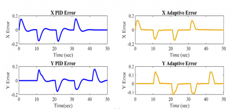
Figure 6 below here is a look at the difference between the use of both controllers (PID and PID adaptive) regarding error.
Figure 6. Rectangular trajectory controller and the difference between the use of both controllers (PID and PID adaptive) regarding error
6.2 Circular trajectory
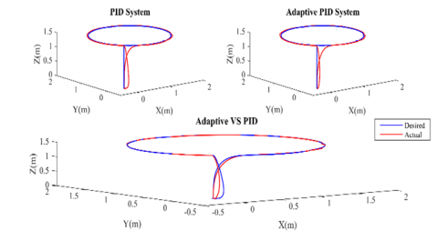
Figure 7 shows the trajectory tracking and comparison between desired track (in blue) and actual track (in red).
Figure 7. Circular trajectory: Using PID controller (upper left corner), using adaptive PID controller (upper right corner), PID vs. adaptive PID (bottom center)
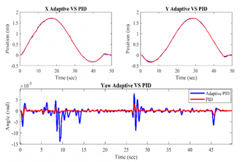
While Figure 8 shows comparison between PID (in red) and adaptive PID (in blue) of X and Y positions also the yaw angle (ψ).
Figure 8. Comparison between PID (in red) and adaptive PID (in blue) of X and Y positions also the yaw angle (ψ) in circular trajectory
And when looking at Figure 9 below in terms of error, we clearly see the differences that occur when using two different controllers (PID and adaptive PID).
Figure 9. Circular trajectory controller and the difference between the use of both controllers (PID and PID adaptive) regarding error
In this paper we studied the kinematic and dynamic models of quadrotor and discussed the Newton-Euler and Euler-Lagrange equations, we also presented two control method of quadrotor which are PID and adaptive PID. We used MATLAB Simulink to test the efficiency of those two control methods in stabilizing and guiding the quadrotor to follow two different trajectories (rectangular and circular). The results of the simulation indicated that both controllers were capable of guiding the quadrotor along the desired path, with the adaptive PID controller reducing position errors more than the normal PID controller, particularly in the circular trajectory.
$C(\Phi, \dot{\Phi})\left[\begin{array}{lll}C_{11} & C_{12} & C_{13} \\ C_{21} & C_{22} & C_{23} \\ C_{31} & C_{32} & C_{33}\end{array}\right]$
$C_{11}=0$
$C_{12}=\left(\mathrm{I}_{\mathrm{yy}}-\mathrm{I}_{\mathrm{zz}}\right)\left(\dot{\theta} \cos (\varphi) \operatorname{sine}(\varphi)+\dot{\psi} \operatorname{sine}(\varphi)^2 \cos (\theta)\right)+\left(\mathrm{I}_{\mathrm{zz}}-\mathrm{I}_{\mathrm{yy}}\right) \dot{\psi} \cos (\varphi)^2 \cos (\theta)-\mathrm{I}_{\mathrm{xx}} \dot{\psi} \cos (\theta)$
$\mathrm{C}_{13}=\left(\mathrm{I}_{\mathrm{zz}}-\mathrm{I}_{\mathrm{yy}}\right) \dot{\psi} \cos (\varphi) \operatorname{sine}(\varphi) \cos (\theta)^2$
$\mathrm{C}_{21}=\left(\mathrm{I}_{\mathrm{zz}}-\mathrm{I}_{\mathrm{yy}}\right)(\dot{\theta} \cos (\varphi) \operatorname{sine}(\varphi)+\dot{\psi} \operatorname{sine}(\varphi) \cos (\theta))+\left(\mathrm{I}_{\mathrm{yy}}-\mathrm{I}_{\mathrm{zz}}\right) \dot{\psi} \cos (\varphi)^2 \cos (\theta)+\mathrm{I}_{\mathrm{xx}} \dot{\psi} \cos (\theta)$
$\mathrm{C}_{22}=\left(\mathrm{I}_{\mathrm{zz}}-\mathrm{I}_{\mathrm{yy}}\right) \dot{\varphi} \cos (\varphi) \operatorname{sine}(\varphi)$
$\mathrm{C}_{23}=-\mathrm{I}_{\mathrm{xx}} \dot{\psi} \operatorname{sine}(\theta) \cos (\theta)+\mathrm{I}_{\mathrm{yy}} \dot{\psi} \operatorname{sine}(\varphi)^2 \operatorname{sine}(\theta) \cos (\theta)+\mathrm{I}_{\mathrm{zz}} \dot{\psi} \cos (\varphi)^2 \operatorname{sine}(\theta) \cos (\theta)$
$\mathrm{C}_{31}=\left(\mathrm{I}_{\mathrm{yy}}-\mathrm{I}_{\mathrm{zz}}\right) \dot{\psi} \cos (\theta)^2 \operatorname{sine}(\varphi) \cos (\varphi)-\mathrm{I}_{\mathrm{xx}} \dot{\theta} \cos (\theta)$
$\mathrm{C}_{32}=\left(\mathrm{I}_{\mathrm{zz}}-\mathrm{I}_{\mathrm{yy}}\right)\left(\dot{\theta} \cos (\varphi) \operatorname{sine}(\varphi) \operatorname{sine}(\theta)+\dot{\varphi} \operatorname{sine}(\varphi)^2 \cos (\theta)\right)+\left(\mathrm{I}_{\mathrm{yy}}-\mathrm{I}_{\mathrm{zz}}\right) \dot{\varphi} \cos (\varphi)^2 \cos (\theta)+\mathrm{I}_{\mathrm{xx}} \dot{\psi} \operatorname{sine}(\theta) \cos (\theta)-\mathrm{I}_{\mathrm{yy}} \dot{\psi} \operatorname{sine}(\varphi)^2 \operatorname{sine}(\theta) \cos (\theta)-\mathrm{I}_{\mathrm{zz}} \dot{\psi} \cos (\varphi)^2 \operatorname{sine}(\theta) \cos (\theta)$
$\mathrm{C}_{33}=\left(\mathrm{I}_{\mathrm{yy}}-\mathrm{I}_{\mathrm{zz}}\right) \dot{\varphi} \cos (\varphi) \sin e(\varphi) \cos (\theta)^2-\mathrm{I}_{\mathrm{yy}} \dot{\theta} \sin e(\varphi)^2 \cos (\theta) \sin e(\theta)-\mathrm{I}_{\mathrm{zz}} \dot{\theta} \cos (\varphi)^2 \cos (\theta) \sin e(\theta)+\mathrm{I}_{\mathrm{xx}} \dot{\theta} \cos (\theta) \sin e(\theta)$
[1] Bouadi, H., Mora-Camino, F. (2018). Direct adaptive backstepping flight control for quadcopter trajectory tracking. In 2018 IEEE/AIAA 37th Digital Avionics Systems Conference (DASC), 2018, pp. 1-8. https://doi.org/10.1109/DASC.2018.8569628
[2] Gao, W.N., Fang, Z. (2012). Adaptive integral backstepping control for a 3-DOF helicopter. In 2012 IEEE International Conference on Information and Automation, 2012, pp. 190-195. https://doi.org/10.1109/ICInfA.2012.6246806
[3] Patel, N., Purwar, S. (2020). Adaptive neural control of quadcopter with unknown nonlinearities. In 2020 IEEE International Conference on Computing, Power and Communication Technologies (GUCON), pp. 718-723. https://doi.org/10.1109/GUCON48875.2020.9231153
[4] Li, T., Zhang, Y., Gordon, B.W. (2012). Nonlinear fault-tolerant control of a quadrotor UAV based on sliding mode control technique. IFAC Proceedings, 45(20): 1317-1322. https://doi.org/10.3182/20120829-3-MX-2028.00056
[5] Razinkova, A., Gaponov, I., Cho, H.C. (2014). Adaptive control over quadcopter UAV under disturbances. In 2014 14th International Conference on Control, Automation and Systems (ICCAS 2014), pp. 386-390. http://dx.doi.org/10.1109/ICCAS.2014.6988027
[6] Bouadi, H., Cunha, S.S., Drouin, A., Mora-Camino, F. (2011). Adaptive sliding mode control for quadrotor attitude stabilization and altitude tracking. In 2011 IEEE 12th international symposium on computational intelligence and informatics (CINTI), pp. 449-455. http://dx.doi.org/10.1109/CINTI.2011.6108547
[7] Czakó, B.G., Kósi, K. (2017). Novel method for quadcopter controlling using nonlinear adaptive control based on robust fixed point transformation phenomena. In 2017 IEEE 15th International Symposium on Applied Machine Intelligence and Informatics (SAMI), pp. 000289-000294. https://doi.org/10.1109/SAMI.2017.7880320
[8] Eltayeb, A., Rahmat, M.F., Basri, M.A.M., Eltoum, M.A.M., El-Ferik, S. (2020). An improved design of an adaptive sliding mode controller for chattering attenuation and trajectory tracking of the quadcopter UAV. IEEE Access, 8: 205968-205979. http://dx.doi.org/10.1109/ACCESS.2020.3037557
[9] Rashid, M.I., Akhtar, S. (2022). Adaptive control of a quadrotor with unknown model parameters. In Proceedings of 2012 9th International Bhurban Conference on Applied Sciences & Technology (IBCAST), pp. 8-14. https://doi.org/10.1109/IBCAST.2012.6177518
[10] Muthusamy, P.K., Garratt, M., Pota, H., Muthusamy, R. (2021). Real-time adaptive intelligent control system for quadcopter unmanned aerial vehicles with payload uncertainties. IEEE Trans. Ind. Electron., 69(2): 1641-1653. http://dx.doi.org/10.1109/TIE.2021.3055170
[11] Darwito, P.A., Wahyuadnyana, K.D. (2022). Performance examinations of quadrotor with sliding mode control-neural network on various trajectory and conditions. Mathematical Modelling of Engineering Problems, 9(3): 707-714. https://doi.org/10.18280/mmep.090317
[12] Santoso, F., Garratt, M.A., Anavatti, S.G. (2015). Fuzzy logic-based self-tuning autopilots for trajectory tracking of a low-cost quadcopter: A comparative study. In 2015 International Conference on Advanced Mechatronics, Intelligent Manufacture, and Industrial Automation (ICAMIMIA), pp. 64-69. http://dx.doi.org/10.1109/ICAMIMIA.2015.7508004
[13] Eltayeb, A., Rahmat, M.F., Eltoum, M.A.M., Basri, M.A.M. (2019). Adaptive fuzzy gain scheduling sliding mode control for quadrotor UAV systems. In 2019 8th International Conference on Modeling Simulation and Applied Optimization (ICMSAO), pp. 1-5. https://doi.org/10.1109/ICMSAO.2019.8880438
[14] Sarabakha, A., Fu, C.H, Kayacan, E., Kumbasar, T. (2017). Type-2 fuzzy logic controllers made even simpler: From design to deployment for UAVs. IEEE Transactions on Industrial Electronics, 65(6): 5069-5077. https://doi.org/10.1109/TIE.2017.2767546
[15] Dydek, Z.T., Annaswamy, A.M., Lavretsky, E. (2012). Adaptive control of quadrotor UAVs: A design trade study with flight evaluations. IEEE Transactions on Control Systems Technology, 21(4): 1400-1406. https://doi.org/10.1109/TCST.2012.2200104
[16] Fernando, T., Chandiramani, J., Lee, T., Gutierrez, H. (2011). Robust adaptive geometric tracking controls on SO (3) with an application to the attitude dynamics of a quadrotor UAV. In 2011 50th IEEE conference on decision and control and European control conference, 2011, pp. 7380-7385. https://doi.org/10.1109/CDC.2011.6161306
[17] Mohammadi, M., Shahri, A.M. (2013). Decentralized adaptive stabilization control for a quadrotor UAV. In 2013 First RSI/ISM International Conference on Robotics and Mechatronics (ICRoM), pp. 288-292. https://doi.org/10.1109/ICRoM.2013.6510121
[18] Li, M., Zuo, Z.Y, Sun, D.L, Wang, C.Y, Wang, W. (2016). Trajectory tracking of a quadrotor helicopter based on ℒ 1 adaptive control. In 2016 IEEE Chinese Guidance, Navigation and Control Conference (CGNCC), pp. 1887-1892. https://doi.org/10.1109/CGNCC.2016.7829077
[19] Celen, B., Oniz, Y. (2018). Trajectory tracking of a quadcopter using fuzzy logic and neural network controllers. In 2018 6th International Conference on Control Engineering & Information Technology (CEIT), pp. 1-6. https://doi.org/10.1109/CEIT.2018.8751810
[20] Rosales, C., Soria, C., Carelli, R., Rossomando, F. (2017). Adaptive dynamic control of a quadrotor for trAajectory tracking. In 2017 International Conference on Unmanned Aircraft Systems (ICUAS), pp. 547-553. https://doi.org/10.1109/ICUAS.2017.7991492
[21] Bhatia, A.K., Jiang, J., Zhen, Z.Y, Ahmed, N., Rohra, A. (2019). Projection modification based robust adaptive backstepping control for multipurpose quadcopter UAV. IEEE Access, 7: 154121-154130. .https://doi.org/10.1109/ACCESS.2019.2946416
[22] Mahmood, T.S., Lutfy, O.F. (2022). A wavelet neural network-based NARMA-L2 feedforward controller using genetic algorithms to control nonlinear systems. Journal Européen des Systèmes Automatisés, 55(4): 439-447. https://doi.org/10.18280/jesa.550402