Raghu Karigowda* | Prameela Kumari Nagaraj
© 2022 IIETA. This article is published by IIETA and is licensed under the CC BY 4.0 license (http://creativecommons.org/licenses/by/4.0/).
OPEN ACCESS
On-grid approaches for DOA estimation majorly exhibits the problem of grid mismatch. Coarse grid leads to reduced estimation accuracy and dense grid leads to increased algorithm complexity and performance degradation due to highly correlated array manifold matrix. In this paper, a fixed off-grid DOA estimation algorithm is proposed to overcome this grid mismatch problem. Firstly, a sparsity based linear interpolation model for array manifold matrix is proposed to avoid the above limitation by introducing a bias parameter into the estimation framework. To solve this model, an Auto-regression (1) (AR (1)) based sparse Bayesian learning algorithm is proposed. To exploit the temporal correlation property of unknown DOA spatial spectrum in a MMV case, we develop this AR (1) model along with SBL to estimate the unknown DOA spectrum and expectation maximization (EM) framework to update the hyper-parameters. The results section shows that the proposed algorithm enjoys good estimation resolution and accuracy in the cases of fewer snapshots available, highly correlated signal sources, very low SNR and very closely spaced sources.
direction of arrival estimation, sparse Bayesian learning, auto-regression model, linear interpolation
In recent years, the direction of arrival estimation problem has been a hot-topic in the areas of research like statistical array signal processing. The main objective of this problem is to accurately estimate the incoming signal directions at the receiver end or simply to locate the signal sources. Extensive survey on this topic indicates the use of a uniform linear array of antenna elements or sensors at the receiver to provide solution to this problem of DOA estimation [1]. The transmitted signals in the case of far-field sources impinge on this linear array of sensors. The signal samples collected by this linear array possess the mathematical property from which the direction information of the signals can be estimated.
Generally, in array signal processing, if the signal directions are known, the signal itself can be received without the loss of information. This concept is reversed in DOA estimation algorithms where, from the received signal samples the direction information of signals is estimated [1]. DOA estimation algorithm finds its application in variety of areas such as RADAR, navigation, SONAR, seismology, wireless mobile communications and many more [2].
There are a quiet plenty of such DOA estimation algorithm in the literature which has its own good performance parameters and at the same time the shortfalls. Such algorithms can be widely categorized into two major techniques including conventional subspace based methods [3-5] and sparse based methods [6]. MUSIC [3] is the most appreciated subspace based algorithm in the field of DOA estimation, which is the simplest form of all the algorithms giving acceptable estimation accuracy, but suffers in the case of highly correlated signal sources. Many algorithms like IMUSIC [7], RMUSIC [7], ESPRIT [4] and other extended versions of MUSIC were developed to improve the performance of the conventional MUSIC algorithm in later years. After the induction of sparse signal reconstruction (SSR) in the field of compressive sensing, an era of sparsity based DOA estimation algorithms has emerged [8]. These algorithms modified the problem of DOA estimation into a SSR problem [9-13]. As these SSR problems work on finite signal measurements, need of a grid, which contains a set of all possible directions (0° ≤ θ ≤ 180°) is required. From the set of single measurement vector (SMV) or multiple measurement vector (MMV) of received signals, a sparse DOA spatial spectrum can be estimated from the help of the defined on-grid possible DOAs.
The first group of SSR modeled DOA estimation algorithms are proposed based on lp -norm (0≤p≤1) convex optimization techniques [9]. These techniques yield good accuracy of estimation but suffer in the case of highly correlated columns of array steering matrix. A dimensionality reduction technique [6] using singular value decomposition (SVD) is applied for l1-norm framework. This resulting l1-SVD algorithm is the major breakthrough in the research of sparse based DOA estimation because of its less complexity and good estimation resolution. When a fine grid size is selected to achieve high accuracy of estimation, the performance of l1-SVD algorithm deteriorates due to highly correlated columns of array steering matrix, which is a result of compact grid set.
In the second group of SSR modeled DOA estimation algorithms, there comes Sparse Bayesian Learning (SBL) and its extensions [11, 12] in the spot light. Sparse Bayesian inference [14] was first proposed for linear regression problem and was applied to DOA estimation problem [15, 16] using on-grid approaches. It is clear [11] that SBL based algorithms are better than lp-norm techniques even in the case of highly correlated signal sources and the column of array steering matrix. These on-grid SBL algorithms uses Bayesian inference to estimate the sparse DOA spectrum through posterior mean and covariance estimation of the unknown parameter by assuming Gaussian probability distribution for the prior and likelihood functions [17, 18]. It is clearly shown [19] that SBL approach enjoys less convergence error when compared to l1-SVD approach. But, for all these SBL and its extension techniques [11-19], defining of a suitable grid set and grid size is very much essential. The algorithm’s resolution and accuracy directly depend on this on-grid set values. A coarse grid set defined, might not include the true DOAs in it, leading to poor estimation accuracy and a fine grid set leads to highly correlated columns of array steering matrix, which in turn makes the algorithm complex and very slow. This grid mismatch problem can be solved by the off-grid technique proposed [20-22]. In off-grid methods, a grid is required for the DOA estimation, but the true DOAs need not to be present in the defined grid set.
Even though the true DOAs are not part of the grid set, they can be estimated accurately by estimating the bias offset values of true DOAs from its nearest grid set value. The algorithms proposed [22] introduces off-grid method in SBL to solve DOA estimation problem by utilizing the first order Taylor series expansion on the columns of the array steering matrix. The authors [20] propose linear interpolation method instead of Taylor expansion like [22], to improve the performance in-terms of accuracy.
In this paper, an Auto-regressive model for the sparse, spatial DOA spectrum is developed in the MMV case. By using linear interpolation as in the case of [20], an off-grid algorithm for DOA estimation is established, involving a SBL-EM solver. The AR (1) property of the spatial DOA spectrum [20] is not exploited resulting in the deterioration of estimation accuracy during low SNR and highly correlated signal sources [23, 24]. This problem is overcome in this paper, where the AR (1) model developed in the beginning of the proposed framework exploits the correlation property through AR (1) coefficient as one of the updating hyper-parameter. Further, the paper has been organized as follows: Section II describes the proposed AR (1) modeling of the DOA estimation problem. Section III showcases the experimental results carried out on the proposed algorithm. Section IV concludes the paper with major summarized points on the simulation results along with advantages, disadvantages and the future work.
In this paper, following are the notations considered: Bold letters are used to represent vectors and matrices, with uppercase letters for matrices and lowercase letters for vectors.
Consider an uniform linear array (ULA) of M sensors with an array manifold matrix of $A(\theta)=\left[a\left(\theta_1\right), a\left(\theta_2\right) \ldots a\left(\theta_K\right)\right]$, by assuming K number of far-field signals impinging on the ULA. Each column vector of A(θ) contains the time-delay information of the Kth signal received at the ULA by taking first sensor in the ULA as the [25]. The general representation of the array manifold matrix is as shown below:
$A(\theta)=\left[\begin{array}{ccc}1 & 1 & 1 \\ e^{-j \beta d \sin \theta_1} & e^{-j \beta d \sin \theta_2} & e^{-j \beta d \sin \theta_K} \\ \vdots & \vdots & \vdots \\ e^{-j \beta d(M-1) \sin \theta_1} & e^{-j \beta d(M-1) \sin \theta_2} & e^{-j \beta d(M-1) \sin \theta_K}\,\,\,\, \end{array}\right]$
where, β=2π/λ and λ is the wavelength of the received signal, d is the spacing between the array elements.
Let $\mathrm{s}(\mathrm{t})=\left[s_1(t), s_2(t) \ldots s_K(t)\right]^T$ be the K number of signals impinging on the ULA. Modeling an ULA mathematically, the signal vector received by the ULA sensors is given by Eq. (1).
$y(t)=A(\theta) s(t)+w(t)$ (1)
where, t = t1, t2 …tL represents the number of snapshots with t=1 for SMV case and t>1 for MMV case. w(t) is the complex independent white Gaussian noise introduced by the sensors and the environmental conditions with zero mean and a variance of $\sigma^2$. To model the DOA estimation problem, selecting a grid set of all possible values of angle space from 0° to 180° is essential. Considering N as the number of grids, let $\bar{\theta}=\left[\bar{\theta}_1, \bar{\theta}_2 \ldots \bar{\theta}_N\right]^T$ be a finite set of grid angle values. $\theta=\left[\theta_1, \theta_2 \ldots . \theta_K\right]^T$ being the true DOAs will be a sub-set of $\bar{\theta}$, only if the true DOAs exactly lie on the chosen grid set. The model in Eq. (1) can be re-written as in Eq. (2) by considering the atoms of array manifold matrix corresponding to all the N grid set values.
$y(t)=A(\bar{\theta}) \bar{s}(t)+w(t)$ (2)
In Eq. (2), the $\bar{s}(t)$ is a sparse vector, which mostly contains zeros and K number of non-zero values corresponding to the rows that are associated with the true DOAs. The solution to this DOA estimation problem in model Eq. (2) is to estimate $\bar{s}(t)$ with the only knowledge of y(t) i.e. the array received signal vector in the presence of noise w(t) [26]. Extending the model in Eq. (2) to MMV case, we get the Eq. (3).
$Y=A \bar{S}+W$ (3)
where, $Y=\left[y\left(t_1\right), y\left(t_2\right) \ldots \ldots y\left(t_L\right)\right]$ is array received matrix, $\bar{s}=\left[\bar{s}\left(t_1\right), \bar{s}\left(t_2\right) \ldots \ldots \bar{s}\left(t_L\right)\right]$ is the sparse spatial signal matrix and $W=$ $\left[w\left(t_1\right), w\left(t_2\right) \ldots \ldots w\left(t_L\right)\right]$ is the sensor measurement noise matrix. The grid set $\bar{\theta}$ chosen must be dense enough to make sure that it consists of the true DOAs. This dense grid makes the algorithm computationally very complex and also results in highly correlated columns of array manifold matrix A. This makes most of the sparse based signal recovery techniques to fail. This grid mismatch problem can be overcome by adopting off-grid methodology [22].
2.1 Linearly interpolated signal model
In off-grid technique a grid set is still needed but the true DOAs need not to be strictly lying on the chosen grid. There will be an offset or bias between the true DOAs and its nearest value in the grid set [27, 28]. Using linear interpolation technique to model the array manifold matrix A as given in Eq. (4) will introduce the bias parameter into the DOA estimation model. Along with the estimation of the sparse spatial spectrum, one should also estimate the bias parameter, which alleviates the performance degradation caused by the grid mismatch problem.
$\bar{a}\left(\theta_n\right)=\left(1-\rho_n\right) a\left(\bar{\theta}_n^{(l)}\right)+\rho_n a\left(\bar{\theta}_n^{(r)}\right)$ (4)
where, $\rho_n$ is the $\mathrm{n}^{\text {th }}$ bias parameter, $\bar{\theta}_n^{(l)}$ and $\bar{\theta}_n^{(r)}$ are the angles present in the grid set adjacent to the true DOA $\theta_n$ from left and right respectively. Replacing each column of A as per the interpolation given in Eq. (4), a new array manifold matrix $\bar{A}$ is formed as given in Eq. (5).
$\bar{A}=A(1: N-1) \operatorname{diag}(1-\rho)+A(2: N-1) \operatorname{diag}(\rho)$ (5)
where, $\rho=\left[\rho_1, \rho_2, \ldots \rho_{N-1}\right]^T$ and A(m:n) indicates that mth to nth column of A matrix. With this interpolation, the signal model in Eq. (3) gets modified to equation shown in Eq. (6).
$Y=\bar{A} \bar{S}+W$ (6)
2.2 Auto-regression based sparse Bayesian learning algorithm
To solve the model in Eq. (6), we make the assumption that the unknown signal matrix $\bar{S}$ (in MMV case) have the same sparsity structure i.e, common sparsity [29]. Each row of $\bar{S}$ corresponds to the signal parameter received in the direction present in the corresponding row of the chosen grid set vector $\bar{\theta}$. Except for the K number of rows, all the other rows of $\bar{S}$ will be having entirely zeros. Those each non-zero row of $\bar{S}$ will also have the same correlated signal parameter values and satisfies Auto-regression (AR(1)) model given by Eq. (7).
$\bar{S}_{i, t+1}=\beta \bar{S}_{i, t}+\sqrt{1-\beta^2} n_{i, t}$ for $i=1,2 \ldots N$ and $t=t_1, t_2 \ldots t_L$ (7)
where, the AR coefficient $\beta \in(-1,1)$ and assuming $n_{i, t}$ and $\bar{S}_{i, t}$ both are Gaussian random processes with probability distribution function of $\mathcal{N}\left(0, \alpha_i\right)$. This Gaussian assumption for the unknown, noise variance and other hyper-parameters are motivated by the SBL framework [14-19]. The value of $\alpha_i$ as zero indicates the variance of ith row of $\bar{S}$ matrix is zero; which means the entries of that complete row is zero promoting sparsity. With this AR(1) model assumption for $\bar{S}$, the joint probability distribution function of $\bar{S}$ is given by Eq. (8).
$\mathrm{P}\left(\overline{\mathrm{S}}_{\mathrm{i}} ; \alpha_{\mathrm{i}}, \beta\right)=\mathcal{N}_s\left(0, \mathrm{R}_{\mathrm{i}}\right) \quad ; \forall \mathrm{i} \in[1,2, \ldots \mathrm{N}]$ (8)
where, $R_i=\alpha_i B^{-1}$ is the covariance matrix of $\bar{S}_i$. B is a Toeplitz matrix of AR coefficient $\beta$ defined by Eq. (9).
$B \equiv\left[\begin{array}{cccc}1 & \beta & \cdots & \beta^{L-1} \\ & \vdots & \ddots & \vdots \\ \beta^{L-1} & \beta^{L-2} & \cdots & 1\end{array}\right]^{-1}$ (9)
By converting MMV model in Eq. (6) into block sparse SMV model, we get Eq. (10).
$y=\phi \bar{s}+\epsilon$ (10)
where, $y=\operatorname{vec}\left(Y^T\right) \in \mathbb{R}^{M L X 1}, \phi=\bar{A} \otimes I_L, e=\operatorname{vec}\left(W^T\right)$ and $\bar{s}=\operatorname{vec}\left(\bar{S}^T\right) \in \mathbb{R}^{N L X 1}$. Sparse Bayesian Inference [14,15] can be applied to solve this model in Eq. (10) by the assuming the Gaussian probability distribution function for the likelihood of the model Eq. (10) as given in Eq. (11).
$\mathrm{P}\left(\mathrm{y} \mid \bar{s} ; \sigma^2, \rho\right) \sim \mathcal{N}\left(\phi \bar{s}, \sigma^2 \mathrm{I}\right)$ (11)
As followed in our previous work [19], the prior of $\bar{S}$ is given by:
$\mathrm{P}\left(\bar{s} ; \alpha_{\mathrm{i}}, \beta\right)=\prod_{i=1}^N P\left(\bar{s}_i ; \alpha_{\mathrm{i}}, \beta\right)$
$\mathrm{P}\left(\bar{s} ; \alpha_{\mathrm{i}}, \beta\right) \sim \mathcal{N}\left(0, \Sigma_0^{-1}\right)$ (12)
where, $\Sigma_0 \equiv \Gamma \otimes B$ and $\Gamma=\operatorname{diag}\left\{\alpha_1^{-1} \ldots \alpha_N^{-1}\right\}$. The posterior function will also be a Gaussian distribution given by Eq. (13).
$P\left(\bar{s} \mid y ; \sigma^2, \Gamma, \beta, \rho\right) \sim \mathcal{N}\left(\mu_{\bar{s}}, \Sigma_{\bar{s}}\right)$ (13)
where, the posterior mean and covariance matrix are given by Eq. (14) and Eq. (15) respectively.
$\mu_{\bar{s}}=\sigma^{-2} \Sigma_{\bar{s}} \phi^{\mathrm{T}} \mathrm{y}$ (14)
$\Sigma_{\bar{s}}=\left[\sigma^{-2} \phi^{\mathrm{T}} \phi+\Sigma_0\right]^{-1}$ (15)
The hyper-parameters like $\sigma^2, \Gamma, \beta$ and $\rho$ are updated iteratively using Expectation Maximization (EM) framework as followed [19] by treating $\bar{s}$ as the hidden variable. The cost function $\mathrm{Q}$ in the EM framework is given by Eq. (16).
$Q=E_{\bar{s} \mid y}\left\{\log P\left(y, \bar{s} ; \alpha, \sigma^2, \beta, \rho\right)\right\}$ (16)
To estimate the variance $\alpha$, the above Q function reduces to Eq. (17).
$Q(\alpha)=L \log (|\Gamma|)-\operatorname{Tr}\left[(\Gamma \otimes B)\left(\hat{\Sigma}_{\bar{s}}+\hat{\mu}_{\bar{s}} \hat{\mu}_{\bar{s}}^T\right)\right]$ (17)
The $\widehat{\mu}_{\bar{s}}$ and $\widehat{\Sigma}_{\bar{s}}$ are evaluated from the previous values of the hyper-parameters. Differentiating Eq. (17) with respect to $\alpha_i$(i=1,2..N) and equating it to zero we get the update equation for $\alpha_i$ as in Eq. (18).
$\alpha_i{ }^{(n e w)}=\frac{1}{L} \operatorname{Tr}\left[B\left(\hat{\Sigma}_{\bar{s}_{i i}}+\hat{\mu}_{\bar{s}_i} \hat{\mu}_{\bar{s}_i}{ }^T\right)\right]$ (18)
where, $\hat{\mu}_{\bar{s}_i}$ refers to the ith row of $\hat{\mu}_{\bar{s}}$ vector and $\widehat{\Sigma}_{\bar{s}_{i i}}$ refers to the ith row and ith column of the $\widehat{\Sigma}_{\bar{s}}$ matrix.
To estimate the AR coefficient $\beta$, the Q function can be written as:
$Q(\beta)=N \log (|\mathrm{B}|)-\operatorname{Tr}\left[(\Gamma \otimes B)\left(\hat{\Sigma}_{\bar{s}}+\hat{\mu}_{\bar{s}} \hat{\mu}_{\bar{s}}^T\right)\right]$ (19)
Differentiating Eq. (19) with respect to $\beta$ and equating it to zero, we get:
$\beta^{(\text {new })}=\beta^{(o l d)}+\eta \operatorname{Tr}\left[(\Gamma \otimes(B F B))\left(\hat{\Sigma}_{\bar{s}}+\hat{\mu}_{\bar{s}} \hat{\mu}_{\bar{s}}{ }^T\right)-N B F\right]$ (20)
where, $F=\partial\left(B^{-1}\right) / \partial \beta$ and η is a small step size which can be determined by classic backtracking method.
$\sigma^2$ can be updated by maximizing the EM cost function given in Eq. (21).
$Q\left(\sigma^2, \rho\right)=-M L \log \sigma^2-\sigma^{-2}\left[\left\|y-\phi \hat{\mu}_{\bar{s}}\right\|^2+\sigma^2\left[N L-\operatorname{Tr}\left(\hat{\Sigma}_{\bar{s}} \Sigma_0\right)\right]\right]$ (21)
Hence the update equation of $\sigma^2$ is given by Eq. (22).
$\sigma^{2^{(\text {new })}}=\frac{\left\|y-\phi \hat{\mu}_{\bar{s}}\right\|^2+\sigma^{2(\text { old })}\,\,\,\, \left[N L-\operatorname{Tr}\left(\hat{\Sigma}_{\bar{s}} \Sigma_0\right)\right]}{M L}$ (22)
Differentiating Eq. (21) with respect to ρ and equating it to zero gives the update equation for ρ as follows:
$\rho=U^{-1} V$ (23)
where,
$U=\mathcal{R}\left\{\left(L \hat{\Sigma}_{\bar{s}}+\hat{\mu}_{\bar{s}} \hat{\mu}_{\bar{s}}^T\right) \odot\left(\phi_{b f}^T \phi_{b f}\right)\right\}$ (24)
$V=\mathcal{R}\left\{\operatorname{diag}\left[\phi_{b f}^T\left(y-\phi_f \hat{\mu}_{\bar{s}}\right) \hat{\mu}_{\bar{s}}^T-L \phi_{b f}^T \phi_{b f} \hat{\Sigma}_{\bar{s}}\right]\right\}$ (25)
$\phi_{b f}=\phi\left(I_b-I_f\right)$ (26)
$\phi_f=\phi I_f$ (27)
$I_b=\left[0_{(N-1) \times 1}, I_{N-1}\right]^T$
$I_f=\left[I_{(N-1)}, 0_{(N-1) \times 1}\right]^T$
Once the EM framework converges, the ρ obtained as a sparse vector contains many zero entries and a few non-zero values. These non-zero values indicate the relationship between the true DOAs and the corresponding $\bar{\theta}_n^{(l)}$ present in the chosen grid set. The true DOAs which are not on the grid set can be accurately determined by the Eq. (28).
$\hat{\theta}_n=\bar{\theta}_n^{(l)}+\delta \rho_n$ (28)
where, $\delta$ is the grid spacing or interval and the suffix ‘n’ represents the nth non-zero element of ρ. That is the number of non-zero elements of ρ is equal to the number signal sources impinging on the ULA. In summary, the proposed off-grid AR(1) based SBL algorithm for DOA estimation (OGARSBL) is presented in Table 1.
Table 1. The proposed OGARSBL DOA estimation algorithm
|
Input Parameters: Y (MxL), A (MxN) Output Parameter: Estimated DOAs $\hat{\theta}$ |
|
Initialize the hyper-parameters $\sigma^2, \alpha, \rho, \beta$. Repeat Estimate $\mu_{\bar{s}}$ using Eq. (14). Estimate $\Sigma_{\bar{s}}$ using Eq. (15). Update $\alpha_i$using Eq. (18). Update β using Eq. (20). Update $\sigma^2$ using Eq. (22). Update ρ using Eq. (27), Eq. (26), Eq. (25), Eq. (24) and Eq. (23) in sequence. Until convergence Estimate true DOAs using Eq. (28). |
In this section, the simulation results of the proposed algorithm (OGARSBL) are presented along with the performance comparison of proposed algorithm with the previous standard and conventional algorithms like l1-SVD [6], MUSIC [3], MVDR [30] and OGSBI [20]. All of these simulations are carried out on MATLAB 2019 platform with minimum 1000 to 2000 Monte-Carlo simulations.
Before the discussion on the simulation results, some of the initializations and performance parameters used for the experimentation are defined below.
The root mean square (RMSE) is the parameter used to analyze the proposed algorithm’s estimation accuracy and is defined as $R M S E=\sqrt{\sum_{t=1}^T\left\|\hat{\theta}^{(t)}-\theta^{(t)}\right\|_2^2 / T K}$ where, T is the number of trials, K is the number of signal sources, $\hat{\theta}^{(t)}$ and $\theta^{(t)}$ are the estimated and true DOA sets of the K signals in tth trial respectively. The simulations are carried out on a 10-element uniform linear array with an element spacing less than the wavelength of the signal. The hyper-parameters are initialized as follows: $\alpha=[1,1, \ldots . .1], \rho=0, \beta=1, \sigma^2=0.1 \times\|Y\|_F^2 / M L$. The proposed algorithm OGARSBL terminate when $\left(\left|\alpha^{(i+1)}-\alpha^{(i)}\right| /\left|\alpha^{(i)}\right|\right)<10^{-4}$.
3.1 Spatial spectrum comparisons
In this subsection, the DOA spatial spectrum of our proposed algorithm is compared with other standard DOA estimation algorithms.
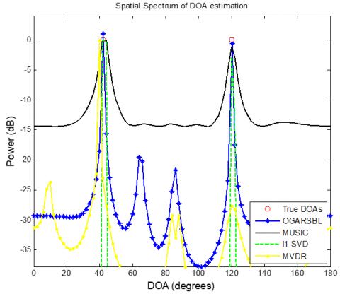
Case 1: Considering an ULA with M=8 number of sensors with an element spacing of d≥λ/2. Let us assume two far-field signal sources with true DOAs of 42.37° and 120.23° impinge on the ULA. The grid size chosen for this case is N=91 i.e, with a grid interval of 2° covering the entire angle space from 0o to 180°. The number of snapshots considered for the measured signal is 200. The SNR of received signal is considered as 0dB. Figure 1(a) shows the DOA spatial spectrum obtained as a simulation result of various algorithms along with the proposed OGARSBL, l1-SVD and MUSIC exhibits two peaks at the angles near to 40o and 120°. Figure 1(b) and Figure 1(c) shows the point view of the DOA peaks. It can be observed that OGARSBL algorithm produces peaks at 42.56° and 120.2°, whereas all the other algorithms show the peak point at 42° and 120°. This is due to the on-grid approach followed by other algorithms.
Case 2: In this case, the effect of reducing the number of snapshots on the DOA peaks is shown. For the same parameters considered in Case 1, the number of snaphots L is reduced to 50. Figure 2(a) shows the increase in number of redundant side peaks for false DOAs, but at the true DOAs the peaks are maximum and indicating the DOAs as 42.4° and 120.5° as shown in Figure 2(b) and Figure 2(c).
It can also be observed that the other previous algorithms show the peaks at 44° and 122°. Even though the number of side peaks increased for OGARSBL compared to other algorithms, the estimation accuracy at the two maximum peaks is high.
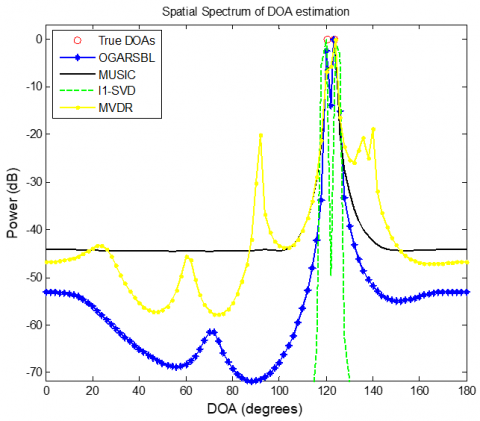
Case 3: This case shows the performance of proposed algorithm for a single snapshot of received signal (i.e., L=1) by keeping all other parameters as same as Case 1. Figure 3 shows the clear peak point view with a DOA peak at 45.69° achieved by OGARSBL algorithm and a DOA peak at 48° achieved by l1-SVD, whereas MVDR and MUSIC does not produce any peaks at the true DOA. The same thing is true even for the true DOA of 120.23°.
(a)
(b)
(c)
Figure 1. (a): DOA spatial spectrum for L=200; (b): DOA spectrum showing true DOA of 42.37° for L=200; (c): DOA spectrum showing true DOA of 120.23° for L=200
(a)
(b)
(c)
Figure 2. (a): DOA spatial spectrum for L=50; (b): DOA spectrum showing true DOA as 42.37° for L=50; (c): DOA spectrum showing true DOA of 120.23° for L=50
Figure 3. DOA spectrum showing true DOA of 42.37° for L=1
(a)
(b)
Figure 4. (a): DOA spatial spectrum for correlated cases; (b): DOA spectrum point view for correlated sources
(a)
(b)
Figure 5. (a): DOA spectrum for closely spaced signal sources; Figure 5(b): Point view of Figure 5(a)
Case 4: When the two signal sources that are impinging on the ULA are correlated with each other, the simulation results are shown in Figure 4(a) and Figure 4(b) with the same parameters as mentioned in Case 1. As seen in the figures, only OGARSBL and l1-SVD produces DOA peaks higher than -5dB of power level at true DOAs, whereas all other algorithms do not indicate highest peaks at true DOAs. Figure 4(b) shows that OGARSBL estimates the DOAs as 42.22° and 120.7°, whereas l1-SVD estimates the DOAs as nearest point in the chosen grid set i.e., 44° and 120°. Hence, even in the case of highly correlated signal sources, OGARSBL does not fail to produce highly accurate results.
Case 5: Consider two signals impinging on the ULA are very closely spaced to each other with true DOAs being 120.58° and 123.67°, with all other same parameters mentioned in Case 1. Figure 5(a) and Figure 5(b) shows clear two separate peaks at the true DOAs produced by l1-SVD and OGARSBL and other algorithms like MVDR and MUSIC shows a single peak and fails to differentiate between the closely spaced two signal sources. As the considered true DOAs in this case is very much nearer to the chosen grid set (i.e., 120° and 124°), both OGARSBL and l1-SVD performances are observed as almost similar, but l1-SVD performance deteriorates when the actual true DOA values are far from the grid set values.
(a)
(b)
Figure 6. (a): DOA spatial spectrum showing OGSBI and OGARSBL performances; (b): Point view of Figure 6(a)
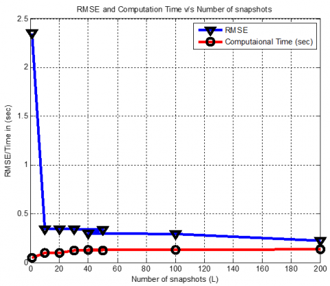
Figure 7. RMSE and computation time v/s number of snapshots
Figure 8. Performance comparison of RMSE v/s SNR
Figure 9. Performance comparison of RMSE v/s SNR for correlated signal sources
Case 6: In this case, the proposed OGARSBL algorithm is compared with an algorithm based on off-grid approach referred as OGSBI [20]. Figure 6(a) and Figure 6(b) show the DOA spectrum obtained by these two algorithms for the same parametric data mentioned in Case 1 with the true DOAs being 43.34° and 121.58°. In Figure 6(b), the DOA estimated by OGARSBL is 43.39°, where as OGSBI estimates it as 44°, even though the off-grid approach is used in OGSBI, since the correlation property present in the MMV model of DOA estimation is not exploited as it is done in the OGARSBL algorithm.
3.2 Performance comparisons
Considering the same parametric values as mentioned in the Case 1, Figure 7 shows the performance of OGARSBL algorithm in terms of Root mean square error (RMSE) and computational time with respect to variation in number of snapshots L. As the number of snapshots increases, the RMSE decreases to a minimum value, at the same time, the computational time required by the algorithm also increases, suggesting a trade-off between both. Figure 8 shows the performance of various algorithms in terms of RMSE v/s SNR. The proposed algorithm observes very low RMSE for a SNR range of -10dB to -5dB compared to other standard algorithms. In high SNR ranges of 5dB to 20dB, OGARSBL performs similar to that of OGSBI algorithm. Figure 9 shows the performance comparison for the case of highly correlated signal sources indicating the better performance of proposed OGARSBL when compared to the other standard algorithms.
In this paper, the DOA estimation problem was solved using off-grid approach by employing Sparse Bayesian Learning-Expectation maximization framework. Sparse Signal reconstruction technique was employed along with a bias parameter related to linear interpolation to accurately estimate the true DOAs which may or may not be present in the selected grid set. To solve this interpolated model, an Auto-Regression (1) based sparse Bayesian learning with expectation maximization framework was proposed. The AR (1) coefficient introduced into the SBL technique helps to exploit the temporal correlation property of the unknown spatial spectrum, which increases the estimation accuracy and the success rate in the case of highly correlated signal sources. The extensive simulation results shown in the previous section indicates the performance of the proposed algorithm in all the different scenarios and dimensions. The resolution obtained by the proposed algorithm in the case of very closely spaced signal sources enjoys greater performance when compared to the other standard and conventional DOA estimation algorithms.
We sincerely thank REVA University, faculty and student friends for extending their support in all aspects for the completion of this work and paper. We also thank our parents and the almighty for all the moral support and encouragement.
|
Variables |
|
|
y |
Array received signal vector |
|
A |
Array manifold matrix/Vandermode matrix |
|
s |
Signal vector impinging on the ULA |
|
w |
Array noise vector |
|
M |
Number of array elements in the ULA |
|
N |
Grid size |
|
L |
Number of snapshots |
|
K |
Number of signal sources impinging on the ULA |
|
Greek symbols |
|
|
$\alpha$ |
Variance of the signal |
|
$\beta$ |
AR coeffecient |
|
$\phi$ |
Array manifold matrix after AR modeling |
|
θ |
Angle of arrival of the signal |
|
µ |
Mean of the signal |
|
ρ |
Bias parameter of linear interpolation |
|
$\sigma^2$ |
Noise variance |
|
δ |
Grid spacing |
|
$\Sigma$ |
Covariance matrix of the signal |
|
Operators |
|
|
diag(.) |
Diagonal entries of a matrix |
|
$ |
Normal gaussian distribution function |
|
E{.} |
Expectation operator |
|
Vec(.) |
Vectorization operator |
|
$\otimes$ |
Kronecker product |
|
Tr[.] |
Trace of a matrix |
|
$ |
Real part of a complex variable |
[1] Krim, H., Viberg, M. (1996). Two decades of array signal processing research: The parametric approach. IEEE Signal Processing Magazine, 13(4): 67-94. http://dx.doi.org/10.1109/79.526899
[2] Liu, C., Antypenko, R., Sushko, I., Zakharchenko, O., Wang, J. (2021). Marine distributed radar signal identification and classification based on deep learning. Traitement du Signal, 38(5): 1541-1548. https://doi.org/10.18280/ts.380531
[3] Schmidt, R. (1986). Multiple emitter location and signal parameter estimation. IEEE Transactions on Antennas And Propagation, 34(3): 276-280. http://dx.doi.org/10.1109/TAP.1986.1143830
[4] Roy, R., Kailath, T. (1989). ESPRIT-estimation of signal parameters via rotational invariance techniques. IEEE Transactions on Acoustics, Speech, and Signal Processing, 37(7), 984-995. http://dx.doi.org/10.1109/29.32276
[5] Capon, J. (1969). High-resolution frequency-wavenumber spectrum analysis. Proceedings of the IEEE, 57(8): 1408-1418. http://dx.doi.org/10.1109/PROC.1969.7278
[6] Malioutov, D., Cetin, M., Willsky, A.S. (2005). A sparse signal reconstruction perspective for source localization with sensor arrays. IEEE Transactions on Signal Processing, 53(8): 3010-3022. http://dx.doi.org/10.1109/TSP.2005.850882
[7] Raghu, K. (2018). Performance evaluation & analysis of direction of arrival estimation algorithms using ULA. 2018 International Conference on Electrical, Electronics, Communication, Computer, and Optimization Techniques (ICEECCOT), pp. 1467-1473. http://dx.doi.org/10.1109/ICEECCOT43722.2018.9001455
[8] Cotter, S.F., Rao, B.D., Engan, K., Kreutz-Delgado, K. (2005). Sparse solutions to linear inverse problems with multiple measurement vectors. IEEE Transactions on Signal Processing, 53(7): 2477-2488. http://dx.doi.org/10.1109/TSP.2005.849172
[9] Hyder, M.M., Mahata, K. (2010). Direction-of-arrival estimation using a mixed ℓ2,0 norm approximation. IEEE Transactions on Signal processing, 58(9): 4646-4655. http://dx.doi.org/10.1109/TSP.2010.2050477
[10] Wipf, D., Nagarajan, S. (2010). Iterative reweighted ℓ1 and ℓ2 methods for finding sparse solutions. IEEE Journal of Selected Topics in Signal Processing, 4(2): 317-329. http://dx.doi.org/10.1109/JSTSP.2010.2042413
[11] Yang, Z., Li, J., Stoica, P., Xie, L. (2018). Sparse methods for direction-of-arrival estimation. In Academic Press Library in Signal Processing, 7: 509-581. http://dx.doi.org/10.1016/B978-0-12-811887-0.00011-0
[12] Zhang, Z., Rao, B.D. (2013). Extension of SBL algorithms for the recovery of block sparse signals with intra-block correlation. IEEE Transactions on Signal Processing, 61(8): 2009-2015. http://dx.doi.org/10.1109/TSP.2013.2241055
[13] Raghu, K., Prameela, K.N. (2019). On-grid adaptive compressive sensing framework for underdetermined DOA estimation by employing singular value decomposition. International Journal of Innovative Technology and Exploring Engineering, 8(11): 3076-3082. http://dx.doi.org/10.35940/ijitee.K2433.0981119
[14] Tipping, M.E. (2001). Sparse Bayesian learning and the relevance vector machine. Journal of Machine Learning Research, 1(Jun): 211-244.
[15] Wipf, D.P., Rao, B.D. (2004). Sparse Bayesian learning for basis selection. IEEE Transactions on Signal processing, 52(8): 2153-2164. http://dx.doi.org/10.1109/TSP.2004.831016
[16] Zhang, Z., Rao, B.D. (2011). Sparse signal recovery with temporally correlated source vectors using sparse Bayesian learning. IEEE Journal of Selected Topics in Signal Processing, 5(5): 912-926. http://dx.doi.org/10.1109/JSTSP.2011.2159773
[17] Liu, Z.M., Huang, Z.T., Zhou, Y.Y. (2011). Direction-of-arrival estimation of wideband signals via covariance matrix sparse representation. IEEE Transactions on Signal Processing, 59(9): 4256-4270. http://dx.doi.org/10.1109/TSP.2011.2159214
[18] Huang, Q., Zhang, G., Fang, Y. (2017). DOA estimation using block variational sparse Bayesian learning. Chinese Journal of Electronics, 26(4): 768-772. http://dx.doi.org/10.1049/cje.2017.04.004
[19] Raghu, K., Prameela, K.N. (2021). Bayesian learning scheme for sparse DOA estimation based on maximum-a-posteriori of hyperparameters. International Journal of Electrical and Computer Engineering, 11(4): 3049-3058. http://dx.doi.org/10.11591/ijece.v11i4.pp3049-3058
[20] Wu, X., Zhu, W.P., Yan, J. (2015). Direction of arrival estimation for off-grid signals based on sparse Bayesian learning. IEEE Sensors Journal, 16(7): 2004-2016. http://dx.doi.org/10.1109/JSEN.2015.2508059
[21] Zhang, Y., Ye, Z., Xu, X., Hu, N. (2014). Off-grid DOA estimation using array covariance matrix and block-sparse Bayesian learning. Signal Processing, 98: 197-201. http://dx.doi.org/10.1016/j.sigpro.2013.11.022
[22] Yang, Z., Xie, L., Zhang, C. (2012). Off-grid direction of arrival estimation using sparse Bayesian inference. IEEE Transactions on Signal Processing, 61(1): 38-43. http://dx.doi.org/10.1109/TSP.2012.2222378
[23] Schoenecker, S., Luginbuhl, T. (2016). Characteristic functions of the product of two Gaussian random variables and the product of a Gaussian and a gamma random variable. IEEE Signal Processing Letters, 23(5): 644-647. http://dx.doi.org/10.1109/LSP.2016.2537981
[24] Donoho, D.L., Elad, M. (2003). Optimally sparse representation in general (nonorthogonal) dictionaries via ℓ1 minimization. Proceedings of the National Academy of Sciences, 100(5): 2197-2202.
[25] Ganguly, S., Ghosh, J., Srinivas, K., Kumar, P.K., Mukhopadhyay, M. (2019). Compressive sensing based two-dimensional DOA estimation using L-shaped array in a hostile environment. Traitement du Signal, 36(6): 529-538. https://doi.org/10.18280/ts.360608
[26] Alabideen, L.Z., Al-Dakkak, O., Khorzom, K. (2021). Hybrid reweighted optimization method for gridless direction of arrival estimation in heteroscedastic noise environment. Mathematical Modelling of Engineering Problems, 8(1): 125-133. https://doi.org/10.18280/mmep.080116
[27] Liu, J., Xie, Q. (2008). Inequalities involving Khatri-Rao products of positive semidefinite Hermitian matrices. International Journal of Information and Systems Sciences, 1: 30-40.
[28] Zhang, Z., Rao, B.D. (2011). Sparse signal recovery with temporally correlated source vectors using sparse Bayesian learning. IEEE Journal of Selected Topics in Signal Processing, 5(5): 912-926. http://dx.doi.org/10.1109/JSTSP.2011.2159773
[29] Al-Shoukairi, M., Schniter, P., Rao, B.D. (2017). A GAMP-based low complexity sparse Bayesian learning algorithm. IEEE Transactions on Signal Processing, 66(2): 294-308. http://dx.doi.org/10.1109/TSP.2017.2764855
[30] Salama, A.A., Ahmad, M.O., Swamy, M.N.S. (2016). Underdetermined DOA estimation using MVDR-weighted LASSO. Sensors, 16(9): 1549. http://dx.doi.org/10.3390/s16091549