Analytical Study of Instability Phenomenon Using Laplace Transform

The fingering phenomenon has been discussed, which occurred in two immiscible phase flow through the homogeneous porous media. It has been reported that the simply investigated the unidirectional flow of immiscible fluids in the large medium. The variation in the values of pressure, saturations and speed of fluid in a single space direction corresponds to the movement direction [1].

In case of thicker porous medium, the vertical components of velocity of fluid could not be ignored. For the porous medium, the analyzed value of forces represents the interfaces, that are generally distorted (encroachment) the fronts. The front is referred to the zone of medium in which saturation of injected phase sharply rises. The encroachment on the scale of the front is known as tongue phenomenon. If it occurred on the smaller scale, then it’s referred as fingering [2]. The condition of the stability of instability is directed to the encroachment. It has been reported that the instabilities depend on the mobility ratio (M). It is also reported that the mobility ratio (M) higher than 1 is more precisely for the appearing of instabilities [3]. The injected fluids that are more transportable than native fluid could be causes of harmful instabilities. The difference in viscosities of flowing fluids causes the occurrence of the phenomenon of fingering. Most of the reports showed that the capillary pressure has been neglected. Further Borana et al. [4] have included the capillary pressure in the analyzed of fingers. Scheidegger [1] has given a review on the instabilities of displacement fronts in porous media and represented the most practically significant method for the oil production in the oil reservoir engineering. Hence, at the time of oil recovery process the fingers should be stabilized [4].

Therefore, the authors should be attention towards the study of finger phenomenon with capillary pressure. The individual pressure of two flowing phases may be replaced by their common mean pressure and the behavior of the fingers. These can be determined by the statistical treatment. Darcy’s law (2003), the equation of continuity and certain basic assumptions yields given a nonlinear partial differential equation for the motion of saturation of injecting fluid [5].

The earlier reports have been investigated the instabilities in displacement process through the homogeneous porous media by various methods. In the earlier study, we reported the analytic solution of instability phenomena using Fourier Transform method [6]. However, no report prevails for using Laplace transform for solving the problem of instability phenomena [7-9].

Here, we demonstrate the analytical solution of instability phenomenon by using Laplace Transform method. It is also discussed the correlation and confirm the observed results of the analytical methods with simulation results.

3.1 Fundamental equation

From the validity of Darcy’s law, let assumed that the seepage velocity of water and oil are (V_w) and (V_o) respectively and can be written as:

$V_{w}=-\frac{k_{w}}{\mu_{w}} k \frac{\partial P_{w}}{\partial x}$        (1)

$V_{o}=-\frac{k_{o}}{\mu_{o}} k \frac{\partial P_{o}}{\partial x}$         (2)

where, k is the permeability of the homogeneous medium, k_w, P_w and μ_w are represents the relative permeability, pressure and viscosity of water similarly, k_o, P_o and μ_o are the relative permeability, pressure and viscosity of oil.

Let assume that the relative permeability of water and oil are the functions of water saturation (S_w) and oil saturation (S_o), respectively.

The equation of continuity can be written as:

$\varphi \frac{\partial S_{w}}{\partial t}+\frac{\partial V_{w}}{\partial x}=0$      (3)

$\varphi \frac{\partial S_{o}}{\partial t}+\frac{\partial V_{o}}{\partial x}=0$        (4)

where, φ is the porosity of the medium, From the definition of phase saturation, the porous medium considered as fully saturated, and it is evident from:

$S_{w}+S_{o}=1$       (5)

The capillary pressure (P_c) is also known as pressure discontinuity of the flowing phases across their common interface and can be written as:

$P_{c}=P_{o}-P_{w}$        (6)

For the determination of the mathematical analysis, assumed for instabilities the standard form of an analytical expression for the relationship between the relative permeability, phase saturation and capillary pressure, is given as:

$k_{w}=S_{w}, k_{0}=S_{0}=1-S_{w}$       (7)

$P_{c}=-\beta S_{w}$       (8)

Here negative sign indicates the direction of water saturation opposite to the capillary pressure and β assumed a constant with smaller parameter.

The value of oil pressure (P_o) is given by [3]:

$P_{o}=\frac{1}{2}\left(P_{o}+P_{w}\right)+\frac{1}{2}\left(P_{o}-P_{w}\right)$

$P_{o}=\bar{P}+\frac{P_{c}}{2}, P_{o}=\frac{1}{2}\left(P_{o}+P_{w}\right)$      (9)

where, $\bar{P}$ is mean pressure and considered as constant.

3.2 Equation of motion for saturation

Equation of motion for the saturation obtained by the substitute the values of V_w from Eq. (1) in Eq. (3) and value of V_o from Eq. (2) in (4), can be written as:

$\varphi \frac{\partial S_{w}}{\partial t}=\frac{\partial}{\partial x}\left[-\frac{k_{w}}{\mu_{w}} k \frac{\partial P_{w}}{\partial x}\right]$      (10)

$\varphi \frac{\partial S_{o}}{\partial t}=\frac{\partial}{\partial x}\left[-\frac{k_{o}}{\mu_{o}} k \frac{\partial P_{o}}{\partial x}\right]$       (11)

From the Eq. (6) and (10), after eliminating the term $\frac{\partial P_{w}}{\partial x}$, we get:

$\varphi \frac{\partial S_{w}}{\partial t}=\frac{\partial}{\partial x}\left[-\frac{k_{w}}{\mu_{w}} k\left\{\frac{\partial P_{o}}{\partial x}-\frac{\partial P_{c}}{\partial x}\right\}\right]$        (12)

From (11) and (12), using Eq. (5), we obtained:

$\frac{\partial}{\partial x}\left[\left\{\frac{k_{o}}{\mu_{o}}+\frac{k_{w}}{\mu_{w}}\right\} k \frac{\partial P_{o}}{\partial x}-\frac{k_{w}}{\mu_{w}} k \frac{\partial P_{c}}{\partial x}\right]=0$       (13)

After integrating the above equation with respect to the x, we get:

$\left[\left\{\frac{k_{o}}{\mu_{o}}+\frac{k_{w}}{\mu_{w}}\right\} k \frac{\partial P_{o}}{\partial x}-\frac{k_{w}}{\mu_{w}} k \frac{\partial P_{c}}{\partial x}\right]=-A$      (14)

where, A is integration constant.

Simplifying the Eq. (14):

$\frac{\partial P_{o}}{\partial x}=-\frac{A}{k\left\{\frac{k_{o}}{\mu_{o}}+\frac{k_{w}}{\mu_{w}}\right\}}+\frac{k_{w}}{\mu_{w}\left\{\frac{k_{o}}{\mu_{o}}+\frac{k_{w}}{\mu_{w}}\right\}} \frac{\partial P_{c}}{\partial x}$       (15)

After simplification the value of $\frac{\partial P_{o}}{\partial x}$ obtained from Eq. (15) and substitute in Eq. (12), we obtained:

$\varphi \frac{\partial S_{w}}{\partial t}=\frac{\partial}{\partial x}\left[\frac{k_{w}}{\mu_{w}} k\left\{-\frac{A}{k\left\{\frac{k_{o}}{\mu_{o}}+\frac{k_{w}}{\mu_{w}}\right\}}+\frac{k_{w}}{\mu_{w}\left\{\frac{k_{o}}{\mu_{o}}+\frac{k_{w}}{\mu_{w}}\right\}} \frac{\partial P_{c}}{\partial x}-\frac{\partial P_{c}}{\partial x}\right\}\right]$

$\varphi \frac{\partial S_{w}}{\partial t}+\frac{\partial}{\partial x}\left[\frac{k_{o}}{\mu_{o}} k \frac{\partial P_{c}}{\partial x} \frac{1}{\left\{1+\frac{k_{o} \mu_{w}}{k_{w} \mu_{o}}\right\}}+\frac{A}{\left\{1+\frac{k_{o} \mu_{w}}{k_{w} \mu_{o}}\right\}}\right]=0$          (16)

Since, from Eq. (9):

$\frac{\partial P_{o}}{\partial x}=\frac{1}{2} \frac{\partial P_{c}}{\partial x}$

The Eq. (14) becomes after substitute the above value:

$A=\left\{\frac{k_{w}}{\mu_{w}}-\frac{k_{o}}{\mu_{o}}\right\} \frac{k}{2} \frac{\partial P_{c}}{\partial x}$       (17)

Now, substituting the value of A in (16), we get:

$\varphi \frac{\partial S_{w}}{\partial t}+\frac{\partial}{\partial x}\left[k \frac{k_{w}}{2 \mu_{w}} \frac{\partial P_{c}}{\partial x}\right]=0$

$\varphi \frac{\partial S_{w}}{\partial t}+\frac{\partial}{\partial x}\left[k \frac{k_{w}}{2 \mu_{w}} \frac{d P_{c}}{d S_{w}} \frac{\partial S_{w}}{\partial x}\right]=0$        (18)

Using Eq. (7), (8) and (18), we get:

$\varphi \frac{\partial S_{w}}{\partial t}-\frac{\beta k k_{w}}{2 \mu_{w}} \frac{\partial^{2} S_{w}}{\partial x^{2}}=0$        (19)

Let consider:

$k=C_{0} \tau \frac{\varphi^{3}}{M_{s}(1-\varphi)^{2}}, \tau=\left(\frac{L}{L_{e}}\right)^{2}$        (20)

where, φ is porosity; M_s is specific surface area; C₀ Kozeny constant; L_e Effective length of the path of the fluid.

From Eqns. (19) and (20), we get:

$\frac{\partial S_{w}}{\partial t}-\frac{\beta C_{0} \tau k_{w} \varphi^{2}}{2 \mu_{w} M_{s}(1-\varphi)^{2}} \frac{\partial^{2} S_{w}}{\partial x^{2}}=0$       (21)

The obtained equation represents the non-linear partial differential equation of motion for the saturation of injected fluid through the homogeneous porous medium.

$P \frac{\partial S_{i}}{\partial t}+\left(\frac{\beta K_{c}}{\delta_{n}}\right) \frac{\partial}{\partial x}\left[\left(P\left(\alpha S_{i}-1\right) \frac{\partial S_{i}}{\partial x}\right)\right]=0[10]$

Let consider the capillary pressure co-efficient is to small enough use for smaller perturbation parameter.

The Eq. (21) becomes a singular perturbation problem equation by multiplying β with highest derivative term. Such the problem with appropriate conditions has been solved by either numerically or analytically.

The set of conditions can be written as:

$S_{w}(0, t)=0, S_{w}(1, t)=1$       (22)

$S_{w}(x, 0)=0$       (23)

Let assume that at x=L, there is no flow because of consider as impermeable limit, i.e.

Let

$X=\frac{x}{L}, T=\frac{C_{0} \tau k_{w} \varphi^{2}}{2 \mu_{w} M_{s}(1-\varphi)^{2} L^{2}} t$

From (21), we get:

$\frac{\partial S_{w}}{\partial T}-\beta \frac{\partial^{2} S_{w}}{\partial X^{2}}=0$      (24)

$S_{w}(0, t)=0, S_{w}(1, t)=1$        (25)

$S_{w}(X, 0)=0$        (26)

The above equations now can be solve using Laplace transform.

3.3 Mathematical solution by using Laplace transform

Now from Eq. (24) we have:

$\frac{\partial S_{w}}{\partial T}=\beta \frac{\partial^{2} S_{w}}{\partial X^{2}}$

With the boundary conditions are S_w(0, t)=0, S_w(1, t)=1 and initial condition is S_w(X, 0)=0.

The solution of above partial differential equation using Laplace transform method [4], From the Laplace transform:

$\left\{\begin{array}{c}\frac{\partial S_{w}}{\partial T}=s \overline{S_{w}}-S_{w}(X, 0) \\ \frac{\partial^{2} S_{w}}{\partial X^{2}}=\frac{\partial^{2} \overline{S_{w}}}{\partial X^{2}}\end{array}\right.$      (27)

Substitute Eq. (27) in to Eq. (24), so we get:

$\beta \frac{\partial^{2} \overline{S_{w}}}{\partial X^{2}}=s \overline{S_{w}}-S_{w}(X, 0)$        (28)

Given initial condition is S_w(X, 0)=0.

So, (28) becomes:

$\beta \frac{\partial^{2} \overline{S_{w}}}{\partial X^{2}}-s \overline{S_{w}}=0$

$\beta \frac{d^{2} \overline{S_{w}}}{d X^{2}}-s \overline{S_{w}}=0$

$\frac{d^{2} \overline{S_{w}}}{d X^{2}}-\frac{s}{\beta} \overline{S_{w}}=0$         (29)

Solution of (3) will be:

$\overline{S_{w}}(X, s)=c_{1} e^{-\sqrt{\frac{s}{\beta}}X}+c_{2} e^{\sqrt{\frac{s}{\beta} }X}$       (30)

where, c₁ and c₂ are arbitrary constants.

By initial conditions, $\overline{S_{w}}(0, s)=L\left\{S_{w}(0, T)\right\}=L\{0\}=0$.

Substitute this value in (30), $c_{1}+c_{2}=0 \Rightarrow c_{1}=-c_{2}$.

So, (30) becomes:

$\overline{S_{w}}(X, s)=c_{2}\left(-e^{-\sqrt{\frac{s}{\beta}}X}+e^{\sqrt{\frac{s}{\beta}} X} \right)$      (31)

Another initial condition, $\overline{S_{w}}(1, s)=L\left\{S_{w}(1, T)\right\}=L\{1\}=\frac{1}{s}$.

Substitute this condition in (31):

$\frac{1}{s}=c_{2}\left(-e^{-\sqrt{\frac{s}{\beta}} X}+e^{\sqrt{\frac{s}{\beta}} X}\right)$

$c_{2}=\frac{1}{2 \operatorname{ssinh}\left(\sqrt{\frac{s}{\beta}}\right)}$      (32)

By using (31) and (32) we can find the value of c₁:

$c_{1}=-\frac{1}{2 \operatorname{ssinh}\left(\sqrt{\frac{s}{\beta}}\right)}$      (33)

Substitute (32) and (33) in (30) we get:

$\overline{S_{w}}(X, s)=-\frac{1}{2 \operatorname{ssinh}\left(\sqrt{\frac{s}{\beta}}\right)} e^{-\sqrt{\frac{s}{\beta} }X}+\frac{1}{2 \operatorname{ssinh}\left(\sqrt{\frac{s}{\beta}}\right)} e^{\sqrt{\frac{s}{\beta} }X}$

$\overline{S_{w}}(X, s)=\frac{\sinh \left(\sqrt{\frac{s}{\beta}} X\right)}{\operatorname{ssinh}\left(\sqrt{\frac{s}{\beta}}\right)}$

By applying Laplace transform, we get the solution:

$S_{w}(X, T)=\sum_{n=0}^{\infty}\left[\operatorname{erf}_{c}\left(\frac{1-x+2 n}{2 \sqrt{T \beta}}\right)-\operatorname{erf}_{c}\left(\frac{1+x+2 n}{2 \sqrt{T \beta}}\right)\right]$

3.4 Simulation

Simulation Programme:

X=0;

X1=0;

temp=0;

temp1=0;

row=0;

col=0;

count=0;

result=zeros(11,4);

for x=0:0.1:1

    row=row+1;

    col=0;

    for t=0.1:0.1:0.4

        col=col+1;

        for n=0:1000           

            X=(1-x+(2*n))/(2*sqrt(t*0.1));

            X1=(1+x+(2*n))/(2*sqrt(t*0.1));

            temp=temp+erfc(X);

            temp1=temp1+erfc(X1);

            X=0;

            X1=0;

        end       

    result(row,col)=temp-temp1;

    temp=0;

    temp1=0;

    end

end

mat=zeros(11,4);

for i=1:11

    for j=1:4

        mat(i,j)=result(12-i,5-j);

    end

end

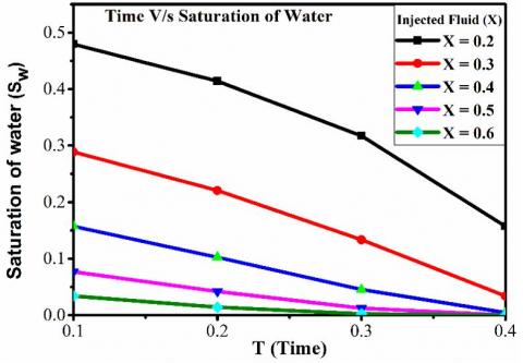
The obtained results from the analytic and simulation of the variation of the saturation in water with respect to the injected fluid and time are shown in Figure 1 and Figure 2, respectively. The results demonstrate that the saturation in water is decreased as increased the injected fluid at fixed time. Whereas, S_w slightly decreases with an increase in time for the fixed amount of injected fluid.

1.jpg

Figure 1. Plot between the injected fluid (%) Vs saturation of water (%)

2.jpg

Figure 2. Variation in saturation in water (%) with respect to the changes in time (sec.)