Pratibha Joshi* | Maheshwar Pathak
© 2022 IIETA. This article is published by IIETA and is licensed under the CC BY 4.0 license (http://creativecommons.org/licenses/by/4.0/).
OPEN ACCESS
Duffing equation can describe many important nonlinear physical systems. In this paper a coupled approach based on quasilinearization and Bessel polynomial collocation method has been suggested to solve nonlinear duffing oscillator equation. The nonlinearity in duffing oscillator can be of various variety. This approach is very efficient, stable and reliable to deal with any kind of nonlinearity. Numerical examples demonstrate the validity and applicability of the approach on various types of nonlinear duffing oscillator equation.
duffing oscillator, quasilinearization, collocation method
Duffing oscillator has been one of the key topics for research for many scientists, engineers and mathematician because of its capacity of modeling various important phenomenon. Researchers have used duffing equation to model free vibrations of a restrained uniform beam with intermediated lumped mass, movement of an oscillating right pendulum with slightly large motions, nonlinear oscillations of many engineering systems e.g. centrifugal governor systems [1], nonlinear vibrations of beams [2], plates [3], fluid flow induced vibrations [4] etc. It has been also used to study behavior of chaotic dynamical systems, magneto-elastic mechanical systems [5].
Since many years mathematicians have been in search of efficient numerical methods [6, 7] to deal with problems arising in engineering. Researchers have been applying variety of numerical methods in solving duffing equation over the years which include variational iteration method [8], differential transform method [9], homotopy perturbation method [10], improved Taylor matrix method [11], Laplace decomposition algorithm [12], modified homotopy perturbation technique [13]. Some researchers have also applied coupled approaches [14-18] which are combination of two or more numerical methods to solve variety of problems. They are combined selectively so that their combination reduces their disadvantages and improve their strength.
In this paper a couple approach is presented which is a combination of quasilinearization and Bessel polynomial collocation method to solve nonlinear duffing equation of the following form:
$y^{\prime \prime}(x)+k_{1} y^{\prime}(x)+k_{2} y(x)+k_{3} f(x, y)=g(x)$ (1)
With initial conditions:
$y(0)=\alpha, y^{\prime}(0)=\beta$ (2)
where, k1, k2, k3, α and β are real constants.
In this approach first the nonlinear duffing Eqns. (1)-(2) is converted into linear form which is further solved by Bessel polynomial collocation method. Generally, the iterative methods work slowly and start getting stuck in the case of complex terms e.g. trigonometric, exponential etc. The proposed method has high accuracy and is very fast. It can deal with complicated nonlinear terms as well as other complex coefficients.
This paper is divided into five sections. In first section, introduction of the present work has been given. In second section, the proposed couple approach is described in detail. In third section, the proposed approach is applied on some numerical examples of duffing equation and the results of current method is compared with that of other numerical methods. In fourth section, the description of error of the current method is mentioned. In the last section, the conclusion of the current work is mentioned.
In this section, we have described the two approached we have combined to develop a coupled approach.
2.1 Quasilinearization
Here the technique of quasilinearization is explained in detail to convert the given nonlinear duffing equation into a linear form.
Let y0(x) be an initial approximation of Eqns. (1) and (2) and sequence of its approximated solution {ym(x)} is determined by the following recurrence relation [19].
$y^{\prime \prime}{ }_{m+1}(x)+k_{1} y_{m+1}^{\prime}(x)+\left\{k_{2}\right.$
$\left.+k_{3} f_{y}\left(y_{m}\right)\right\} y_{m+1}(x)$
$=g(x)-y_{m}^{\prime \prime}-k_{1} y_{m}^{\prime}(x)$
$-k_{2} y_{m}-k_{3} f\left(y_{m}\right)$,
$m=0,1,2 \ldots$ (3)
With boundary conditions:
$y_{m+1}(0)=\alpha, y_{m+1}^{\prime}(0)=\beta$ (4)
Hence, quasilinearization transforms nonlinear form (1) to (2) into linear form (3)-(4). Now we propose to apply Bessel polynomial collocation method [20] to solve linear problem (3)-(4). The details of the method are given in the next subsection.
2.2 Bessel polynomial collocation method
Here we explain Bessel polynomial collocation method using Bessel polynomial matrix method developed by [20].
To find the truncated Bessel polynomial series approximation of the problem (3)-(4) suppose:
$y_{m+1}^{\prime \prime}(x)=\sum_{n=0}^{N} r_{n} J_{n}(x)$ (5)
where, N≥2 (order of the differential Eq. (1)), rn,m; n=0, 1, 2, …, N are unknown coefficients to be determined and Jn(x); n=0, 1, 2,…, N are Bessel polynomials of first kind defined by:
$J_{n}(x)=\sum_{k=0}^{\left[\left[\frac{N-n}{2}\right]\right]} \frac{(-1)^{k}}{k !(k+n) !}\left(\frac{x}{2}\right)^{2 k+n}$
$n=0,1,2, \ldots, \quad 0 \leq x<\infty.$
Now, the matrix form of Bessel polynomials Jn(x) is written as:
$J(x)=X(x) A^{T}$ (6)
where,
J(x)=[J0(x) J1(x) ⋯ JN(x)],
X(x)=[1 x1x2 ⋯ xN].
And if N is odd,
$A=\left[\begin{array}{cccccc}\frac{1}{0 ! 0 ! 2^{0}} & 0 & \frac{-1}{1 ! 1 ! 2^{2}} & \cdots & \frac{(-1)^{\frac{N-1}{2}}}{\left(\frac{N-1}{2}\right) !\left(\frac{N-1}{2}\right) ! 2^{N-1}} & 0 \\ 0 & \frac{1}{0 ! 1 ! 2^{1}} & 0 & \cdots & 0 & \frac{(-1)^{\frac{N-1}{2}}}{\left(\frac{N-1}{2}\right) !\left(\frac{N+1}{2}\right) ! 2^{N}} \\ 0 & 0 & \frac{1}{0 ! 2 ! 2^{2}} & \cdots & \frac{(-1)^{\frac{N-3}{2}}}{\left(\frac{N-3}{2}\right) !\left(\frac{N+1}{2}\right) ! 2^{N-1}} & 0 \\ \vdots & \vdots & \vdots & \ddots & \vdots & \vdots \\ 0 & 0 & 0 & \cdots & \frac{1}{0 !(N-1) ! 2^{N-1}} & 0 \\ 0 & 0 & 0 & \cdots & 0 & \frac{1}{0 ! N ! 2^{N}}\end{array}\right]_{(N+1) \times(N+1)}$.
If N is even,
$A=\left[\begin{array}{cccccc}\frac{1}{0 ! 0 ! 2^{0}} & 0 & \frac{-1}{1 ! 1 ! 2^{2}} & \cdots & 0 & \frac{(-1)^{\frac{N}{2}}}{\left(\frac{N}{2}\right) !\left(\frac{N}{2}\right) ! 2^{N}} \\ 0 & \frac{1}{0 ! 1 ! 2^{1}} & 0 & \cdots & \frac{(-1)^{\frac{N-2}{2}}}{\left(\frac{N-2}{2}\right) !\left(\frac{N}{2}\right) ! 2^{N-1}} & 0 \\ 0 & 0 & \frac{1}{0 ! 2 ! 2^{2}} & \cdots & 0 & \frac{(-1)^{\frac{N-2}{2}}}{\left(\frac{N-2}{2}\right) !\left(\frac{N+2}{2}\right) ! 2^{N}} \\ \vdots & \vdots & \vdots & \ddots & \vdots & \vdots \\ 0 & 0 & 0 & \cdots & \frac{1}{0 !(N-1) ! 2^{N-1}} & 0 \\ 0 & 0 & 0 & \cdots & 0 & \frac{1}{0 ! N ! 2^{N}}\end{array}\right]_{(N+1) \times(N+1)}$
Now, write Eq. (5) in matrix form as:
$y_{m+1}^{\prime \prime}(x)=J(x) Q_{m}$
$Q_{m}=\left[\begin{array}{llll}r_{0, m} & r_{1, m} & \cdots & r_{N, m}\end{array}\right]^{T}$ (7)
From Eqns. (6) and (7), we have:
$y_{m+1}^{\prime \prime}(x)=X(x) A^{T} Q_{m}$ (8)
Integrating Eq. (8) from 0 to x, we get:
$y_{m+1}^{\prime}(x)=y_{m+1}^{\prime}(0)+X X(x) A^{T} Q_{m}$ (9)
where, $X X(x)=\left[\begin{array}{lllll}x & \frac{x^{2}}{2} & \frac{x^{3}}{3} & \cdots & \frac{x^{N+1}}{N+1}\end{array}\right]$.
Integrating Eq. (8) from 0 to x, we get:
$y_{m+1}(x)=y_{m+1}(0)+y_{m+1}^{\prime}(0) x+X X X(x) A^{T} Q_{m}$ (10)
where, $X X X(x)=\left[\begin{array}{lllll}\frac{x^{2}}{1 \times 2} & \frac{x^{3}}{2 \times 3} & \frac{x^{4}}{3 \times 4} & \cdots & \frac{x^{N+2}}{(N+1) \times(N+2)}\end{array}\right]$.
Now, replacing $y_{m}(x), y_{m+1}(x), y_{m+1}^{\prime}(x), y_{m+1}^{\prime \prime}(x)$ in Eqns. (3) and (4) with the values in (8)-(10) we get:
$\begin{aligned} X(x) A^{T} Q_{m}+k_{1}\{&\left.y_{m+1}^{\prime}(0)+X X(x) A^{T} Q_{m}\right\}+\left\{k_{2}\right.\\ &\left.+k_{3} f_{y}\left(y_{m}\right)\right\}\left(y_{m+1}(0)\right.\\ &\left.+y_{m+1}^{\prime}(0) x+X X X(x) A^{T} Q_{m}\right) \\ &=g(x)-y_{m}^{\prime \prime}-k_{1} y_{m}^{\prime}(x) \\ &-k_{2} y_{m}-k_{3} f\left(y_{m}\right), m \\ &=0,1,2 \ldots \end{aligned}$ (11)
Let the collocation points xi be defined as:
$x_{i}=a+\frac{b-a}{N} i, \quad i=0,1,2, \ldots, N$
$0<a \leq x \leq b \leq 1$ (12)
Putting collocation points xi into Eq. (11), we get (N+1) linear equations in terms of (N+1) unknown r0,m, r1,m, …, rN,m as follows:
$\begin{aligned} X\left(x_{i}\right) A^{T} Q_{m}+k_{1} &\left\{y_{m+1}^{\prime}(0)+X X\left(x_{i}\right) A^{T} Q_{m}\right\}+\left\{k_{2}\right.\\ &\left.+k_{3} f_{y}\left(y_{m}\right)\right\}\left(y_{m+1}(0)\right.\\ &\left.+y_{m+1}^{\prime}(0) x_{i}+X X X\left(x_{i}\right) A^{T} Q_{m}\right) \\ &=g\left(x_{i}\right)-y_{m}^{\prime \prime}-k_{1} y_{m}^{\prime}\left(x_{i}\right) \\ &-k_{2} y_{m}-k_{3} f\left(y_{m}\right), \quad m \\ &=0,1,2 \ldots \end{aligned}$ (13)
which can be represented as:
$U Q_{m}=W$ (14)
where,
$U=X_{0} A^{T}+P_{1} X_{1} A^{T}+P_{2} X_{2} A^{T}$
$X_{0}=\left[\begin{array}{ccccc}1 & x_{0} & x_{0}^{2} & \cdots & x_{0}^{N} \\ 1 & x_{1} & x_{1}^{2} & \cdots & x_{1}^{N} \\ \vdots & \vdots & \vdots & \ddots & \vdots \\ 1 & x_{N} & x_{N}^{2} & \cdots & x_{N}^{N}\end{array}\right]_{(N+1) \times(N+1)}$
$X_{1}=\left[\begin{array}{ccccc}\left(x_{0}\right) & \left(\frac{x_{0}^{2}}{2}\right) & \left(\frac{x_{0}^{3}}{3}\right) & \cdots & \left(\frac{x_{0}^{N+1}}{N+1}\right) \\ \left(x_{1}\right) & \left(\frac{x_{1}^{2}}{2}\right) & \left(\frac{x_{1}^{3}}{3}\right) & \cdots & \left(\frac{x_{1}^{N+1}}{N+1}\right) \\ \vdots & \vdots & \vdots & \ddots & \vdots \\ \left(x_{N}\right) & \left(\frac{x_{N}^{2}}{2}\right) & \left(\frac{x_{N}^{3}}{3}\right) & \cdots & \left(\frac{x_{N}^{N+1}}{N+1}\right)\end{array}\right]_{(N+1) \times(N+1)}$
$X_{2}=\left[\begin{array}{cccc}\left(\frac{x_{0}^{2}}{1 \times 2}\right) & \left(\frac{x_{0}^{3}}{2 \times 3}\right) & \cdots & \left(\frac{x_{0}^{N+2}}{(N+1) \times(N+2)}\right) \\ \left(\frac{x_{1}^{2}}{1 \times 2}\right) & \left(\frac{x_{1}^{3}}{2 \times 3}\right) & \cdots & \left(\frac{x_{1}^{N+2}}{(N+1) \times(N+2)}\right) \\ \vdots & \vdots & \ddots & \vdots \\ \left(\frac{x_{N}^{2}}{1 \times 2}\right) & \left(\frac{x_{N}^{3}}{2 \times 3}\right) & \cdots & \left(\frac{x_{N}^{N+2}}{(N+1) \times(N+2)}\right)\end{array}\right]_{(N+1) \times(N+1)}$
$P_{1}=\left[\begin{array}{ccccc}k_{1} & 0 & 0 & \cdots & 0 \\ 0 & k_{1} & 0 & \cdots & 0 \\ \vdots & \vdots & \vdots & \ddots & \vdots \\ 0 & 0 & 0 & \cdots & k_{1}\end{array}\right]_{(N+1) \times(N+1)}$
$P_{2}=\left[\begin{array}{ccccc}k_{2}+k_{3} f_{y}\left(y_{m}\right) & 0 & 0 & \cdots & 0 \\ 0 & k_{2}+k_{3} f_{y}\left(y_{m}\right) & 0 & \cdots & 0 \\ \vdots & \vdots & \vdots & \ddots & \vdots \\ 0 & 0 & 0 & \cdots & k_{2}+k_{3} f_{y}\left(y_{m}\right)\end{array}\right]_{(N+1) \times(N+1)}$
And
$W=\left[\begin{array}{c}g\left(x_{0}\right)-y^{\prime \prime}{ }_{m}-k_{1} y^{\prime}{ }_{m}\left(x_{0}\right)-k_{2} y_{m}-k_{3} f\left(y_{m}\right)-k_{1} \beta-\left\{\left(k_{2}+k_{3} f_{y}\left(y_{m}\right)\right)\left(\alpha+\beta x_{0}\right)\right\} \\ g\left(x_{1}\right)-y_{m}^{\prime \prime}-k_{1} y_{m}^{\prime}\left(x_{1}\right)-k_{2} y_{m}-k_{3} f\left(y_{m}\right)-k_{1} \beta-\left\{\left(k_{2}+k_{3} f_{y}\left(y_{m}\right)\right)\left(\alpha+\beta x_{1}\right)\right\} \\ \vdots \\ g\left(x_{n}\right)-y_{m}^{\prime \prime}-k_{1} y_{m}^{\prime}\left(x_{n}\right)-k_{2} y_{m}-k_{3} f\left(y_{m}\right)-k_{1} \beta-\left\{\left(k_{2}+k_{3} f_{y}\left(y_{m}\right)\right)\left(\alpha+\beta x_{n}\right)\right\}\end{array}\right]_{(N+1) \times 1}$
Now Eq. (14) can be solved by:
$Q_{m}=U^{-1} W$ (15)
Finally, the approximation ym+1(x) can be achieved by replacing g value from Eq. (15) in Eq. (10).
For starting the iteration process of Eq. (13), the initial approximation y0(x) can be taken according to initial conditions. Combining both methods discussed in subsections 2.1 and 2.2, a coupled approach is generated which we call quasilinear Bessel polynomial collocation method (QBPCM). It is applied in solving duffing Eqns. (1)-(2) in this paper.
If $\operatorname{rank}[U]=\operatorname{rank}[U: V]=N+1$ then Qm is uniquely determined i.e. we get unique solution of Eqns. (1)-(2). If $\operatorname{rank}[U]=\operatorname{rank}[U: V]<N+1$ then we find particular solution and if $\operatorname{rank}[U] \neq \operatorname{rank}[U: V]$ then we will not get solution.
For a given m and N, Let Y(x) be the approximated solution of the problem (1)-(2) obtained from QBPCM, where m represents number of approximation in quasilinearization method and (N+1) represents number of collocation points in the Bessel polynomial collocation method. The absolute error in approximated solution Y(x) is estimated as:
$e_{N, m}(x)=|y(x)-Y|$ (16)
where, y(x) is exact solution of problem (1)-(2).
If the exact solution is not available then to perform error analysis, we denote and calculate absolute residual error as follows:
$R e_{N, m}(x)=\mid Y^{\prime \prime}(x)+k_{1} Y^{\prime}(x)+k_{2} Y(x)+k_{3} f(x, y)-g(x) \mid$ (17)
For sufficiently large value of N, $e_{N, m}(x) \rightarrow 0$ and $R e_{N, m}(x) \rightarrow 0$ as $m \rightarrow \infty$ i.e. $Y(x) \rightarrow y(x)$ .
In this section the applicability of the suggested coupled approach has been shown by few numerical examples. All computational work has been performed on Matlab.
Example-1: Let us consider the duffing equation of the following type [11]:
$y^{\prime \prime}+3 y-2 y^{3}=\cos x \sin 2 x \\
with\quad conditions\quad y(0)=0, y^{\prime}(0)=1$. (18)
By applying quasilinearization, the linearized form of Eq. (18) is:
$\begin{aligned}
y_{m+1}^{\prime \prime}(x)+(3-&\left.6 y_{m}^{2}\right) y_{m+1}(x) = \cos x \sin 2 x-4 y_{m}{ }^{3} \\
& m=0,1,2, \ldots
\end{aligned}$ (19)
Now we apply Bessel polynomial collocation method on Eq. (19) as mentioned in section 2. The exact solution of Eq. (18) is y=sin(x). Table 1 shows the absolute error of the solution by the proposed coupled approach for various collocation point N and m=3. Table 1 clearly shows that as we increase collocation points, the absolute error is reducing and accuracy is getting better.
Table 1. The absolute error of solution of Example-1 by proposed approach a m=3
|
x |
N=3 |
N=5 |
N=7 |
|
0.1 |
4.3326×10⁻⁷ |
1.9714×10⁻⁹ |
4.1458×10⁻¹² |
|
0.2 |
2.6072×10⁻⁶ |
8.5622×10⁻⁹ |
1.3494×10⁻¹¹ |
|
0.3 |
6.3277×10⁻⁶ |
1.5300×10⁻⁸ |
2.1025×10⁻¹¹ |
|
0.4 |
1.0357×10⁻⁵ |
2.0078×10⁻⁸ |
2.8136×10⁻¹¹ |
|
0.5 |
1.3443×10⁻⁵ |
2.4388×10⁻⁸ |
3.5090×10⁻¹¹ |
|
0.6 |
1.5052×10⁻⁵ |
2.9500×10⁻⁸ |
4.0913×10⁻¹¹ |
|
0.7 |
1.5717×10⁻⁵ |
3.4221×10⁻⁸ |
4.6751×10⁻¹¹ |
|
0.8 |
1.6900×10⁻⁵ |
3.6986×10⁻⁸ |
5.2446×10⁻¹¹ |
|
0.9 |
2.0300×10⁻⁵ |
4.0280×10⁻⁸ |
5.6556×10⁻¹¹ |
|
1.0 |
2.6513×10⁻⁵ |
4.9719×10⁻⁸ |
6.7456×10⁻¹¹ |
Table 2. Comparison of absolute error of solution of Example 1 by proposed approach with that of other numerical methods
|
x |
Proposed approach |
MVIM |
ITMM |
|
0.0 |
0 |
0 |
0 |
|
0.1 |
1.97×10⁻⁹ |
3.60×10⁻⁷ |
4.62×10⁻⁸ |
|
0.2 |
8.56×10⁻⁹ |
1.02×10⁻⁵ |
6.12×10⁻⁷ |
|
0.3 |
1.53×10⁻⁸ |
2.35×10⁻⁵ |
4.28×10⁻⁷ |
|
0.4 |
2.00×10⁻⁸ |
9.78×10⁻⁷ |
2.29×10⁻⁷ |
|
0.5 |
2.43×10⁻⁸ |
1.60×10⁻⁵ |
4.23×10⁻⁷ |
|
0.6 |
2.95×10⁻⁸ |
3.10×10⁻⁵ |
4.03×10⁻⁷ |
|
0.7 |
3.42×10⁻⁸ |
8.50×10⁻⁵ |
3.32×10⁻⁷ |
|
0.8 |
3.69×10⁻⁸ |
2.19×10⁻⁵ |
5.66×10⁻⁷ |
|
0.9 |
4.02×10⁻⁸ |
3.18×10⁻⁵ |
8.87×10⁻⁶ |
|
1.0 |
4.97×10⁻⁸ |
3.22×10⁻⁵ |
1.43×10⁻⁵ |
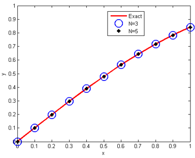
In Table 2 we have compared our results with that of two other numerical methods. We have taken the absolute error of solution at N=5, m=5 by our proposed approach. The other two results are by modified variational iteration method (MVIM) [21] at 20 chebyshev points at 11th iteration and Improved Taylor matrix method (ITMM) for 5th degree Taylor’s polynomial [11]. Through Table 2 it can be seen that the method is in good agreement with the results of other methods even for a low value of N and m. It is obvious that the accuracy will be higher if we take higher number of collocation points N and number of iterations m (Figure 1).
Figure 1. Comparison of exact solution and numerical solution by current method at number of collocation points N=3 and 5 at 5th iteration
Example 2: Consider the duffing equation
$y^{\prime \prime}+0.4 y^{\prime}+1.1 y+y^{3}=2.1 \cos (1.8 x) \\
with\quad conditions\quad y(0)=0.3\quad and\quad y^{\prime}(0)=-2.3$ (20)
The linearized form of Eq. (20) using quasilinearization is:
$\begin{gathered}
y_{m+1}^{\prime \prime}(x)+0.4 y_{m+1}^{\prime}(x)+\left(1.1+3 y_{m}^{2}\right) y_{m+1}=2 y_{m}^{3}+2.1 \cos (1.8 x)
\end{gathered}$. (21)
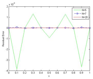
Now after applying Bessel collocation method we get the solution of (20) which can be seen in Table 3 at different points. It is also compared with the solution obtained by other methods [12]. Since the exact solution of (20) is not available, the residual error is evaluated for error analysis. In Table 4 the residual error of the solution obtained for various combination of N and m is demonstrated. The reduction of residual error with increasing collocation point is also displayed by Figure 2.
Figure 2. Reduction of residual error with increasing collocation points N for Example 2
In Figure 2 it can be easily seen that as we take higher collocation points the residual error of Example 2 becomes lower. The error also reduces as we run higher iterations.
Table 3. The comparison of numerical solution of Example-2
|
x |
Present Method |
Laplace Method |
ITMM |
|
0 |
0.3 |
0.3 |
0.3 |
|
0.1 |
0.08358453485 |
0.0835845348 |
0.08358453484 |
|
0.2 |
-0.1050919158 |
-0.105091915 |
-0.1050919158 |
|
0.3 |
-0.2660203036 |
-0.266060303 |
-0.2660203036 |
|
0.4 |
-0.3999779482 |
-0.399977948 |
-0.3999779482 |
|
0.5 |
-0.5083148107 |
-0.508314810 |
-0.5083148107 |
|
0.6 |
-0.5928906891 |
-0.592890689 |
-0.5928906891 |
|
0.7 |
-0.6560655026 |
-0.656065502 |
-0.6560655028 |
|
0.8 |
-0.7006769398 |
-0.700676939 |
-0.7006769399 |
|
0.9 |
-0.7299708506 |
-0.729970850 |
-0.7299708508 |
|
1.0 |
-0.7474760770 |
-0.747476077 |
-0.7474760775 |
Example 3: Consider the damped duffing Equation [11]:
$y^{\prime \prime}(x)+k y^{\prime}=-y^{3}(x) \\
with\quad the\quad initial\quad conditions\quad y\quad(0)=\alpha, y^{\prime}(0)=\beta$ (22)
Here we have considered the case of α=β=k=1. The linearized form of the Eq. (22) from quasilinearization technique is:
$y_{m+1}^{\prime \prime}(x)+y_{m+1}^{\prime}(x)+3 y_{m}^{2} y_{m+1}=2 y_{m}^{3}$ (23)
The residual error of solution of Eq. (22) is shown in Table 4 and is also compared with the results of ITM [11]. The results in Table 4 are taken for N=5 at 10th iterations. The error will be lesser for higher collocation points and number of iterations. The results are promising and in good agreement with that of ITM.
Table 4. Comparison of absolute residual errors of the solution of Example 3 by current method and Improved Taylor matrix method at different x values
|
x |
Current Approach |
ITM |
||
|
N=5 |
N=10 |
5th degree |
8th degree |
|
|
0 |
0 |
0 |
0 |
0 |
|
0.1 |
2.37E-3 |
9.06E-16 |
4.62E-3 |
5.08E-6 |
|
0.2 |
6.56E-16 |
1.88E-17 |
0 |
6.72E-6 |
|
0.3 |
7.05E-4 |
4.49E-17 |
4.54E-3 |
1.45E-6 |
|
0.4 |
1.31E-15 |
7.89E-16 |
0 |
3.82E-6 |
|
0.5 |
4.09E-4 |
1.27E-16 |
7.85E-3 |
0 |
|
0.6 |
2.56E-15 |
8.68E-16 |
0 |
2.62E-5 |
|
0.7 |
4.17E-4 |
5.019E-17 |
5.42E-2 |
3.01E-5 |
|
0.8 |
1.19E-16 |
2.23E-17 |
1.94E-1 |
8.07E-4 |
|
0.9 |
7.87E-4 |
1.50E-15 |
0.46E-1 |
5.68E-3 |
|
1 |
4.15E-15 |
5.67E-17 |
0.93E-1 |
1.22E-2 |
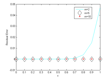
Figure 3. The reduction of residual error with higher number of iterations for Example 3 at 10 collocation points
In Figure 3, it can be seen that as we keep on increasing number of iterations the residual error keeps getting reduced. This is claimed by many iterative methods but when we run higher iterations either the methods start getting very complicated or get stuck. The proposed method is very fast and does not get stuck at higher iterations which is a great advantage of the current method over many iterative methods for the solution of linear [22, 23] and nonlinear problems.
In this paper, the coupled approach QBPCM which is a combination of quasilinearization and Bessel polynomial collocation method is successfully applied to nonlinear duffing equation. The results of QBPCM are also compared to that of other numerical methods to show its efficiency and accuracy. The advantage of this coupled approach is that it is highly accurate, robust and can be applicable to variety of problems. It can easily deal with the nonlinear problems with complicated terms and coefficients and does not take too much computational time and space.
Support from University of Petroleum & Energy Studies (UPES), Dehradun for providing access of MATLAB software to complete this work is gratefully acknowledged. The authors would like to say their sincere thanks to the anonymous reviewers for their valuable comments/suggestions to make this paper more effective.
[1] Younesian, D., Askari, H., Saadatnia, Z., Yazdi, M.K. (2011). Periodic solutions for nonlinear oscillation of a centrifugal governor system using the He’s frequency-amplitude formulation and He’s energy balance method. Nonlinear Science Letters A, 2(3): 143-148.
[2] Ahmadian, M.T., Mojahedi, M., Moeinfard, H. (2009). Free vibration analysis of a nonlinear beam using homotopy and modified Lindstedt-Poincare methods. Journal of Solid Mechanics, 1(1): 29-36.
[3] Bakhtiari-Nejad, F., Nazari, M. (2009). Nonlinear vibration analysis of isotropic cantilever plate with viscoelastic laminate. Nonlinear Dynamics, 56(4): 325-356. http://dx.doi.org/10.1007/s11071-008-9401-z
[4] Srinil, N., Zanganeh, H. (2012). Modelling of coupled cross-flow/in-line vortex-induced vibrations using double Duffing and van der Pol oscillators. Ocean Engineering, 53: 83-97. http://dx.doi.org/10.1016/j.oceaneng.2012.06.025
[5] Guckenheimer, J., Holmes, P. (1983). Nonlinear Oscillations, Dynamical Systems, Springer-Verlag.
[6] Pathak, M., Joshi, P. (2014). High order numerical solutionof a volterra integro-differential equation arising in oscillating magnetic fields using variational iteration method. International Journal of Advanced Science and Technology, 69: 47-56. http://dx.doi.org/10.14257/ijast.2014.69.05
[7] Pathak, M., Joshi, P. (2015). A high order solution of three dimensional time dependent nonlinear convective-diffusive problem using modified variational iteration method. Int. J. Sci. Eng, 8(1): 1-5. http://dx.doi.org/10.12777/ijse.8.1.1-5
[8] He, J.H., Wu, G.C., Austin, F. (2009). The variational iteration method which should be followed. Nonlinear Science Letters A, 1: 1-30.
[9] Tabatabaei, K., Gunerhan, E. (2014). Numerical solution of Duffing equation by the differential transform method. Appl. Math. Applied Mathematics & Information Sciences Letters, 2(1): 1-6. http://dx.doi.org/10.12785/amisl/020101
[10] He, J.H. (1999). Homotopy perturbation technique. Computer Methods in Applied Mechanics and Engineering, 178(3-4): 257-262. http://dx.doi.org/10.1016/S0045-7825(99)00018-3
[11] Bülbül, B., Sezer, M. (2013). Numerical solution of Duffing equation by using an improved Taylor matrix method. Journal of Applied Mathematics, 691614. http://dx.doi.org/10.1155/2013/691614
[12] Yusufoğlu, E. (2006). Numerical solution of Duffing equation by the Laplace decomposition algorithm. Applied Mathematics and Computation, 177(2): 572-580. https://doi.org/10.1016/j.amc.2005.07.072
[13] El-Naggar, A.M., Ismail, G.M. (2016). Analytical solution of strongly nonlinear Duffing oscillators. Alexandria Engineering Journal, 55(2): 1581-1585. http://dx.doi.org/10.1016/j.aej.2015.07.017
[14] Joshi, P., Pathak, M. (2020). A coupled approach to solve the family of Kuramato-Sivashinsky equations. WSEAS Transactions on Mathematics, 19: 91-397. http://dx.doi.org/10.37394/23206.2020.19.40
[15] Pathak, M., Joshi, P. (2018). Application of a coupled approach for the solution of nonlinear singular initial value problems of Lane–Emden type. Astrophysics and Space Science, 363(9): 1-10. http://dx.doi.org/10.1007/s10509-018-3415-x
[16] Joshi, P., Pathak, M. (2019). A coupled approach for solving a class of singular initial value problems of Lane–Emden type arising in astrophysics. In Harmony Search and Nature Inspired Optimization Algorithms, pp. 669-678. http://dx.doi.org/10.1007/s10509-018-3415-x
[17] Pathak, M., Joshi, P. (2021). Modified iteration method for numerical solution of nonlinear differential equations arising in science and engineering. Asian-European Journal of Mathematics, 2050151. http://dx.doi.org/10.1142/S1793557121501515
[18] Pathak, M., Joshi, P. (2021). Thermal analysis of some fin problems using improved iteration method. International Journal of Applied and Computational Mathematics, 7(2): 1-15. http://dx.doi.org/10.1007/s40819-021-00964-0
[19] Bellman, R.E., Kalaba, R.E. (1965). Quasilinearization and Nonlinear Boundary-Value Problems. New York, NY, USA: American Elsevier Publishing.
[20] Yüzbaşı, Ş., Şahı̇n, N., Sezer, M. (2011). Bessel polynomial solutions of high-order linear Volterra integro-differential equations. Computers & Mathematics with Applications, 62(4): 1940-1956. http://dx.doi.org/10.1016/j.camwa.2011.06.038
[21] Gohareeb, F., Babolian, E. (2014). Modified variational iteration method for solving duffing equation. Indian Journal of Scientific Research, 6(1): 25-29.
[22] Pathak, M., Joshi, P. (2019). High-order compact finite difference scheme for Euler–Bernoulli beam equation. In Harmony Search and Nature Inspired Optimization Algorithms, pp. 357-370.
[23] Pathak, M., Joshi, P. (2018). Numerical solution of acoustic wave equation using method of lines. World Journal of Modelling and Simulation, 14(4): 243-256.