Mahmoud Muthana* | Ahmed R. Nasser
© 2022 IIETA. This article is published by IIETA and is licensed under the CC BY 4.0 license (http://creativecommons.org/licenses/by/4.0/).
OPEN ACCESS
Even with the significant progress that has been achieved in monocular depth estimation in recent years, the need for better real-time inference and reduction in computing resources usage associated with the network performance is persistent. In this paper, an enquiry into the efficacy of pruning on depth estimation models is performed. Encoder-decoder model based on the ResNet-50 backbone architecture employing pruning based on channel prioritization is designed to achieve higher performance and prediction speed. This is while attempting to keep a balance in the trade-off between accuracy and performance of the network. The presented approach is trained and evaluated for outdoor scenery on the KITTI dataset to demonstrate the effectiveness and the performance improvement of the presented framework when compared to similar methods. This shows competitive accuracy when compared to state-of-the-art methods and highlights how pruning can speed up inference time by more than 16% and leading to fewer operations compared to the non-pruned model.
computer vision, deep learning, depth estimation
Monocular depth prediction is a complex task in computer vision to predict the depth of objects from a single viewpoint in a particular scene. Numerous applications in fields such as 3D reconstruction [1], robotics [2], and autonomous vehicle perception systems [3] can make use of this task given its fundamental function of determining the scene’s geometrical relationship and acquiring a composition of its spatial structure. Depth prediction methods usually involve range sensors such as LiDARs or in the case of a system involving cameras, various instances and views of the scene to construct a precise estimation which might require sequences of videos from a moving camera [4] or stereo imagery [5]. This causes greater computational resource utilization and more costly equipment to deal with. Thus, the monocular depth estimation model is an important concept to obtain less constrained, more compact, and affordable results for the task.
There are still many difficulties risen from the ill-posed nature of the issue given that there are infinite perspectives of 3D scenes in a 2D image because of the scale ambiguities related to the variations in camera movement speeds and object sizes. Humans can solve these challenges by leveraging local cues such as being aware of occlusion and texture which can also be applied to monocular depth estimators in the learning stage. Earlier techniques in monocular depth estimation relied on handcrafted and probabilistic methods for estimation [6]. But due to the progress made in recent years in convolutional neural networks and deep learning along with the emergence of quality depth datasets enhanced the monocular depth prediction task performance. One of the first methods in this regard was proposed by Eigen et al. [7] by using multi-scale CNNs for depth prediction. First, they carried out global coarse estimation on the scene of the image. Then, the results are sent through an additional CNN to create a more accurate and refined local estimation. Liu et al. [8] presented feature maps up-sampling to enhance the output resolution of the depth prediction.
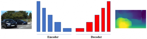
The design of the encoder-decoder is commonly implemented owing to its robust ability to address the depth prediction task (and numerous other tasks such as sentiment analysis [9] and semantic segmentation [10]), the abundance of depth data, and its relatively easy implementation. These techniques usually consist of two main stages. The first stage is an encoder for extracting low-resolution features of the image using networks such as ResNet [11], DenseNet [12] usually for their higher accuracy, or MobileNet [13] for using less resources.
The second stage is the decoder with the objective of up-sampling the features, and fusing them by convolutions to upscale the spatial resolution of the image for improved quality. Among the many methods that can be used in the decoder, the bilinear method was chosen due to its smoother surface results, and less complicated approach when compared to other methods such the bicubic interpolation. It’s achieved by performing linear interpolation in two directions and using the neighboring pixels to estimate the value of the up-sampling block. This is done by adding padded zeros and then calculating the weighted average between two translated pixels for the output value.
Feature extraction networks play an important role in determining the performance of the prediction model through many factors such as the number of layers and the techniques used to build the network which set it apart from other approaches. ResNet is one of the most widely used networks in many fields including image classification, and depth estimation given its innovative architecture which offers the use of the residual blocks to reduce the associated training error in addition to the large number of possible layers that can be added especially in ResNet-50 and ResNet-101 providing 50 and 101 layers respectively.
The encoder-decoder architecture has been used in the depth estimation problem in Ref. [14] where they presented an unsupervised method that estimated depth without the need for prior depth data by relying on the disparity of the right and left images captured by a stereo camera and their novel training loss technique applying consistency between the prediction from each camera during the training. Facil et al. [15] used Camera Aware Multi Scale Convolutions in their encoder-decoder architecture. This allowed the network to estimate the patterns of depth based on the intrinsic values of the camera. The convolution layers capture the camera parameters including the focal length, calibration, angle, etc. Yin and Shi [16] trained an encoder-decoder network to estimate both the surface normals and the depth in order to enforce the geometrical consistency between the planar regions to address the existing blur in the image.
Alhashim and Wonka [17] demonstrated that transfer learning can be leveraged to construct supervised depth estimation with better accuracy. The network employs an encoder-decoder structure based on denseNet-169 backbone architecture. The ImageNet dataset is used to pre-train the network with augmentation techniques to enhance the final estimation of depth while Laina et al. [18] introduced up-sampling feature maps technique to improve output resolution of the estimation depth and built a deeper network based on residual learning. They also introduced the commonly used reverse Huber loss function (berHu) used in this work.
These learning-based prediction models rely on the concept of training a model to predict the depth value for each pixel. The training of these models requires substantial amount of data: more data available during training lead to more reliability in predicting depth. However, this will increase the complexity of these networks which means more parameters, larger model sizes, increased processing resources, and memory utilization required in addition to longer prediction time. This means that increasing the complexity of the model increases the accuracy but at the expense of runtime. Reducing the complexity of the model and computation requirements associated with it while maintaining the same performance has long been a popular issue which necessitates the need for alternative approaches in this regard. Network pruning can be used to mitigate the effects of the mentioned problems to obtain smaller and more efficient networks with faster inference time and less required calculations preferably without significant loss of accuracy [19]. Prior method [20] presented an encoder-decoder based network for depth prediction with a pruning strategy to reduce the model complexity and introduce faster inference time for embedded devices (specifically the NVIDIA Jetson TX2 GPU) using the lightweight MobileNet architecture. Given the work is being done on a lightweight network to accommodate the relatively low processing power of the TX2 GPU and other embedded devices, the trade-off between the accuracy and the size of the model is too big which manifests into a clear compromise in the quality of depth prediction. This work attempts to achieve an improvement in runtime performance and better accuracy results by carrying out the pruning process on a larger backbone network (ResNet-50) in order to create a solution that includes most types of GPUs and hardware. Data augmentation techniques and transfer learning are used to increase the accuracy of the prediction network as shown in the study [17]. This elaborate method can be used on larger systems with a pruning approach [21] based on dynamic pruning that relies on channel prioritization by amplifying and suppressing channels and skipping the unimportant at runtime. The neurons of the model are preserved which will reduce the impact on accuracy while gaining the same efficiency metrics. Hence, the depth estimation network shown in Figure 1 can adequately preserve accuracy and provide better runtime results. The method is evaluated on the KITTI dataset, demonstrating how pruning can reduce the runtime of the network from 90 ms to 76 ms and decrease in the multiply and accumulate operations (MACs) from 3.4G to 2.9G without a significant loss of accuracy.
Thus, to summarize the goal of this paper:
The rest of the paper is organized as follows: The architecture of the depth estimation model and the pruning process are explained in Section 2. Experimental results are showcased and compared with other state-of-the-art methods in Section 3 followed by the conclusion in Section 4.
Figure 1. Encoder-decoder concept
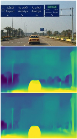
Figure 2. Visualization of the final depth results before and after the pruning process
This section presents the specific details of the depth estimation model shown in Figure 3 starting with the implementation of the encoder-decoder and the network architecture. In Section 2.1, the encoder-decoder design is described and with the overall framework. To improve the accuracy of the depth prediction online data augmentation is applied and reviewed in Section 2.2. The depth loss function is discussed in Section 2.3. In the last section, the pruning technique is explained to improve the performance and increase the efficiency of the system.
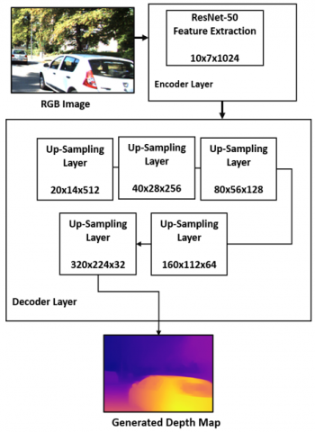
Figure 3. Encoder-decoder architecture
2.1 Encoder-decoder architecture
The general structure of the model is shown in Figure 3. Images consist of spatial information [22] which is minimized by down-sampling the H ×W ×c (c representing the number of channels) image once it gets delivered to the encoder to increase the network’s receptive field and decrease the computational operations. By applying the successive pooling and convolution layers, the image features are extracted. In this model, the encoder is based on the ResNet-50 backbone architecture. It consists of 50 layers with 48 convolutional layers, a max-pooling layer, and a 1 average-pooling layer. The Res-Net model is selected over other encoders such as VGG and DenseNet since it’s been shown that the sparse models tend to better perform in pruning than dense ones [23]. As a substitute for random weight initialization, transfer learning that uses cross-domain knowledge transfer is employed by pretraining the model on the ImageNet dataset since it demonstrated that it can drastically improve the performance of the depth prediction model without any observed downsides as illustrated by the Ref. [17]. The last classifying and average pooling layers of the encoder are discarded so that the decoder can be linked to the encoder with various configurations for the skip connection implemented for the preservation of the details between the decoder and the encoder. The decoding layer consists of 5 bilinear up-sampling layers to establish the depth estimation by up-scaling and fusing the output of the encoder gradually to construct the final depth map. As mentioned earlier, the decoder uses the bilinear method due to its straightforward design and smoother surface compared to the other methods such as the linear interpolation and the bicubic interpolation.
2.2 Data augmentation
As mentioned earlier, depth prediction networks require enormous amount of data in order to obtain good accuracy and produce better depth quality reliably. The more data introduced during the training phase, the better the accuracy. The perpetual limited availability of depth data leads to the exploration of alternative methods such as data augmentation which includes making changes to the existing data in order to be used during training as new instances. Also, employing data augmentation methods for a specific task has been shown to be very effective during the learning stage to minimize the problem of over-fitting and adopt better generalization [24, 25]. These techniques are implemented based on trials and experiments for improved encoder extraction results:
2.3 Depth loss
There are many considerations that can have an effect on the depth prediction performance and the training speed. This leads to many variations in the depth estimation literature for loss functions [14, 20, 26]. Generally, the depth loss function is calculated using the difference between the output of the depth network y and the ground truth of that depth value y*. Reverse Huber loss (BerHu) used in the study [18] is employed because it offers a good balance between the Least Absolute Deviations L1 in Eq. (1) providing the ability to propagate and the Least Square Errors L2 in Eq. (2) which offers lower gradient for the small residuals. The BerHu loss function is shown in Eq. (3)
$L_{1}\left(y^{*}-y\right)=\sum_{i=1}^{n}\left|y_{i}^{*}-y_{i}\right|$ (1)
$L_{2}\left(y^{*}-y\right)=\sum_{i=1}^{n}\left(y_{i}^{*}-y_{i}\right)^{2}$ (2)
$B\left(y^{*}-y\right)=\left\{\begin{array}{c}L_{1}\left(y^{*}-y\right) \text { if }\left(y^{*}-y\right)<c \\ \frac{L_{2}\left(y^{*}-y\right)+c^{2}}{2 c} \text { otherwise }\end{array}\right.$ (3)
2.4 Dynamic pruning process
For optimal results, an established dynamic pruning technique based on channel feature boosting and suppression [21] is modified to prune the ResNet-50. This will not only conserve computational resources but will also reduce the impact on accuracy in the trade-off balance without affecting the neurons like other pruning methods. Deep sequential CNNs are used to prune the parameters so that the information flow can be restricted or amplified allowing the salient information to flow from the important channels while suppressing the rest. To demonstrate the work being done in the original paper, the auxiliary component shown in Figure 4 determines the importance of the channels based on a parametric function p(xl−1) that can be evaluated based on the previous layer xl-1 using Eq. (4).
$p\left(x_{l-1}\right)=w t a_{T}\left(g\left(x_{l-1}\right)\right)$ (4)
The function wta( ) is a k-winner-takes-all function that returns a tensor with zeros (i.e., suppressing the unnecessary channels) for each entry smaller than T which represents the salient channels predicted by the channel saliency predictor g(xl−1).
The spatial dimensions of each channel are reduced to scalar further to preserve computational resources by using the following function in Eq. (5):
$s c\left(x_{l-1}\right)=\frac{s\left(x_{l-1}^{1}\right) s\left(x_{l-1}^{2}\right) \ldots s\left(x_{l-1}^{c}\right)}{H . W}$ (5)
where, H, W represent the height and the width of the channel respectively while c represents the number of channels. g(xl−1) may then can be calculated with the following Eq. (6) Where $\varphi l$ here denotes the weight tensor of the layer.
$g\left(x_{l-1}\right)=\operatorname{sc}\left(x_{l-1}\right) . \varphi l$ (6)
Figure 4. The pruning process
Finally, the dynamically pruned channel can be described with Eq. (7) using the ReLU activation function. Where $\theta_{l}$ representing the weight tensor for the layer.
$f\left(x_{l-1}\right)=p\left(x_{l-1}\right) . \operatorname{nor}\left(\operatorname{conv}\left(x_{l-1}, \theta_{l}\right)\right)$ (7)
From (7) we see that for each layer xl, convolution is performed on the previous layer xl-1 then each channel of features in a population of z is normalized based on Eq. (8):
$\operatorname{nor}(\mathbf{z})=\frac{\mathbf{z}-\operatorname{mean}(\mathbf{z})}{\sqrt{\text { variance }(\mathbf{z})+\in }}$ (8)
where, $\in$ is a small number to avoid division by zero. Normalizing layers are used to stabilize the training and enable learning with faster convergence at a higher rate.
3.1 Implementation details
The method is implemented on the PyTorch [27] framework. The 50-layers ResNet-50 is pretrained on the ImageNet dataset for better initialization and then trained with the parameters according to Table 1. It takes 49 hours for the training of the encoder-decoder network using a GTX 3080 Ti GPU.
Table 1. The training parameters
|
Parameters |
Value |
|
Learning Rate |
0.0001 |
|
Epochs |
30 |
|
Optimizer |
SGD |
|
Batch Size |
8 |
3.2 KITTI dataset & benchmarking suite
The training and the evaluation process of this network are implemented on the KITTI dataset and benchmark suite [28]. KITTI is a publicly available large-scale outdoor scenes dataset for various tasks such as semantic segmentation, optical flow, object detection, and is widely used for depth estimation. It consists of thousands (about 21k images for training) of labeled RGB images with a resolution of 375×1241 of diverse scenes recorded with cameras and depth sensing equipment (such as the Velodyne HDL-64E laser) from outdoor environments and streets with the conforming ground truth depth maps acquired using mounted equipment on a vehicle. It consists of 8 categories including the “car” and “pedestrian“ classes. The depth network is trained using 7k images from 32 training scenes and use 698 images for testing from 29 scenes. The splitting policy is based on the Eigen policy suggested by Liu et al. [8]. The images were resized to a resolution of 640×480 from 375×1241 for improved computation efficiency to generate an output of 320×224.
3.3 Evaluation metrics & results
The assessment of the proposed method is done on outdoor data with the KITTI dataset. The popular metrics employed for the depth prediction task evaluation in literature and this project is presented below. Let yp denote the estimated depth of a pixel in the image, yg is its ground truth and N is the number of pixels in the image.
Root mean squared error (RMS): RMS equation is detailed in Eq. (9):
$\sqrt{\frac{1}{N} \sum_{i=1}^{N}\left(y_{g}^{i}-y_{p}^{i}\right)^{2}}$ (9)
Mean Relative Error (REL): REL equation is detailed in Eq. (10).
$\frac{1}{N} \sum_{i=1}^{N} \frac{\left\|y_{g}^{i}-y_{p}^{i}\right\|}{y_{p}^{i}}$ (10)
RMS log: equation is detailed in Eq. (11).
$\sqrt{\frac{1}{N} \sum_{i=1}^{N}\left\|\log _{10} y_{g}^{i}-\log _{10} y_{p}^{i}\right\|^{2}}$ (11)
Thresholded accuracy(δi): equation is detailed in Eq. (12).
$T>\delta=\max \left(\frac{y_{g}^{i}}{y_{p}^{i}}, \frac{y_{p}^{i}}{y_{g}^{i}}\right)$ (12)
where, $\mathrm{T}=1.25,1.25^{2}, 1.25^{3}$.
Table 2 shows a comparison using these metrics between the proposed method with and without pruning and other state-of-the-art methods. The network is compared to state-of-the-art methods and the results are obtained from original papers.
Table 2. Performance comparison on the KITTI dataset
|
|
Higher is better |
Lower is better |
||||
|
Method/ Metric |
$\delta_{1,25}$ |
$\delta_{1.25^{2}}$ |
$\delta_{1.25^{3}}$ |
REL |
RMS |
RMS log |
|
Saxena et al. [6] |
0.601 |
0.820 |
0.926 |
0.280 |
8.734 |
0.361 |
|
Eigen et al. [7] |
0.702 |
0.898 |
0.967 |
0.203 |
6.307 |
0.282 |
|
Liu et al. [8] |
0.680 |
0.898 |
0.967 |
0.201 |
6.471 |
0.273 |
|
Alhashim and Wonka [17] |
0.886 |
0.965 |
0.986 |
0.093 |
4.170 |
0.171 |
|
Fu et al. [29] |
0.932 |
0.984 |
0.994 |
0.072 |
2.727 |
0.120 |
|
Lee et al. [30] |
0.956 |
0.993 |
0.998 |
0.059 |
2.756 |
0.096 |
|
Proposed Method |
0.865 |
0.940 |
0.964 |
0.096 |
4.714 |
0.184 |
|
Method + pruning |
0.846 |
0.928 |
0.958 |
0.118 |
4.855 |
0.202 |
Experimental results show that pruning can slightly decrease accuracy by lowering the values of δ by 1.5% on average. There’s also an increase of 3.15% on RMS. The method is again compared in Table 3. to the pre-pruned ResNet-50 model to establish how pruning affects the performance and accuracy of the network.
Table 3. Performance comparison between the pruned and unpruned model
|
Method |
MACs |
Runtime |
RMS |
$\delta_{1,25}$ |
|
Without Pruning |
3.4G |
90 ms |
4.714 |
0.865 |
|
After Pruning |
2.9G |
76 ms |
4.855 |
0.846 |
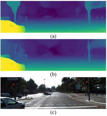
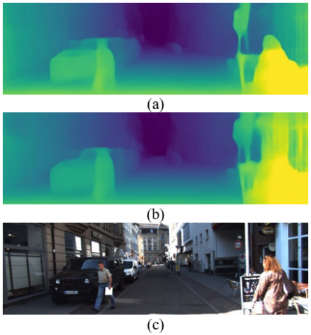
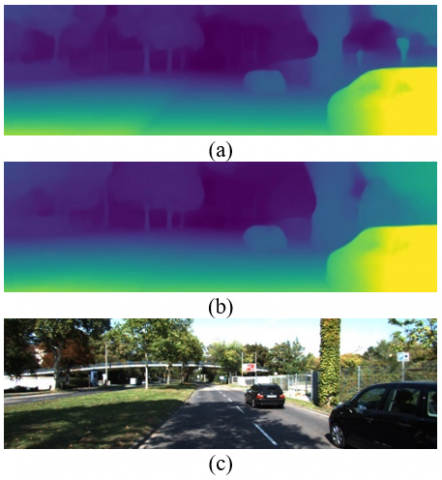
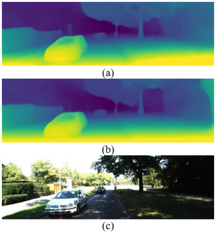
Results from Table 3 reveal an almost 16% difference in inference time compared to the non-pruned model on the GTX 3080 Ti GPU. There’s also an estimated 14.7% reduction in the multiply and accumulate operations (MACs) without any significant loss to accuracy on the accuracy metrics as discussed before RMS (+3.15%), and Thresholded accuracy (-1.5%) compared to the non-pruned model. Figure 5 visualizes the depth maps for each prediction. Colour maps are used to show the difference in depth. Warm-green colors indicate closer distance while colder colors are for farther distances.
Figure 5. Qualitative depth prediction results on KITTI (a) Before pruning results (b) After pruning results (c) Original Image
In this work, a dynamically pruned monocular depth estimation network is implemented using the encoder-decoder architecture by leveraging transfer learning techniques. The method achieves competitive results compared to the state-of-the-art methods on the KITTI dataset. The effects of pruning on the network were investigated and compared to showcase how it can affect the performance of the system. It’s been found that the model performs about 16% faster inference time and uses fewer MACs with insignificant (about 1.5% on average) loss of accuracy due to the trade-off balance that occurs in the pruning process. Demonstrating that pruning can be an effective technique for increasing the performance of the depth network.
[1] Abdul-Kreem, L.I. (2017). Depth estimation and shape reconstruction of a 2D image using NN and Bézier surface interpolation. Iraqi Journal of Computers, Communication, Control & Systems Engineering, 17(1): 24-32.
[2] Hameed, F.S., Alwan, H.M., Ateia, Q.A. (2020). Pose estimation of objects using digital image processing for pick-and-place applications of robotic arms. Engineering and Technology Journal, 38(5): 707-718. https://doi.org/10.30684/etj.v38i5A.518
[3] Wang, Y., Chao, W.L., Garg, D., Hariharan, B., Campbell, M., Weinberger, K.Q. (2019). Pseudo-lidar from visual depth estimation: Bridging the gap in 3d object detection for autonomous driving. In Proceedings of the IEEE/CVF Conference on Computer Vision and Pattern Recognition, pp. 8445-8453. https://doi.org/10.1109/CVPR.2019.00864
[4] Mahmood, S.S., Saud, L.J. (2020). An efficient approach for detecting and classifying moving vehicles in a video based monitoring system. Engineering and Technology Journal, 38(6): 832-845. http://doi.org/10.30684/etj.v38i6A.438
[5] Furukawa, Y., Hernández, C. (2015). Multi-view stereo: A tutorial. Foundations and Trends® in Computer Graphics and Vision, 9(1-2): 1-148. http://doi.org/10.1561/0600000052
[6] Saxena, A., Chung, S., Ng, A. (2005). Learning depth from single monocular images. Advances in Neural Information Processing Systems.
[7] Eigen, D., Puhrsch, C., Fergus, R. (2014). Depth map prediction from a single image using a multi-scale deep network. Advances in Neural Information Processing Systems, 3: 2366-2374. https://doi.org/10.48550/arXiv.1406.2283
[8] Liu, F., Shen, C., Lin, G. (2015). Deep convolutional neural fields for depth estimation from a single image. In Proceedings of the IEEE Conference on Computer Vision and Pattern Recognition, pp. 5162-5170. https://doi.org/10.48550/arxiv.1411.6387
[9] Albayati, A.Q., Ameen, S.H. (2020). A method of deep learning tackles sentiment analysis problem in Arabic texts. Iraqi Journal of Computers, Communications, Control and Systems Engineering, 20(4): 9-20. https://doi.org/10.33103/uot.ijccce.20.4.2
[10] Abdul-Kreem, L.I., Abdul-Ameer, H. K. (2020). Object tracking using motion flow projection for pan-tilt configuration. Int. J. Electr. Comput. Eng., 10(5): 4687-4694.
https://doi.org/10.11591/IJECE.V10I5.PP4687-4694
[11] He, K., Zhang, X., Ren, S., Sun, J. (2016). Deep residual learning for image recognition. In Proceedings of the IEEE Conference on Computer Vision and Pattern Recognition, pp. 770-778. https://doi.org/10.48550/arxiv.1512.03385
[12] Huang, G., Liu, Z., Van Der Maaten, L., Weinberger, K.Q. (2017). Densely connected convolutional networks. In Proceedings of the IEEE Conference on Computer Vision and Pattern Recognition, pp. 4700-4708. https://doi.org/10.1109/CVPR.2017.243
[13] Howard, A.G., Zhu, M., Chen, B., et al. (2017). Mobilenets: Efficient convolutional neural networks for mobile vision applications. arXiv preprint arXiv:1704.04861. https://doi.org/10.48550/arxiv.1704.04861
[14] Godard, C., Mac Aodha, O., Brostow, G.J. (2017). Unsupervised monocular depth estimation with left-right consistency. In Proceedings of the IEEE Conference on Computer Vision and Pattern Recognition, pp. 270-279. https://doi.org/10.1109/CVPR.2017.699
[15] Facil, J.M., Ummenhofer, B., Zhou, H., Montesano, L., Brox, T., Civera, J. (2019). CAM-Convs: Camera-aware multi-scale convolutions for single-view depth. In Proceedings of the IEEE/CVF Conference on Computer Vision and Pattern Recognition, pp. 11826-11835. https://doi.org/10.1109/CVPR.2019.01210
[16] Yin, Z., Shi, J. (2018). Geonet: Unsupervised learning of dense depth, optical flow and camera pose. In Proceedings of the IEEE Conference on Computer Vision and Pattern Recognition, pp. 1983-1992. https://doi.org/10.1109/CVPR.2018.00212
[17] Alhashim, I., Wonka, P. (2018). High quality monocular depth estimation via transfer learning. arXiv Preprint arXiv:1812.11941. https://doi.org/10.48550/arxiv.1812.11941
[18] Laina, I., Rupprecht, C., Belagiannis, V., Tombari, F., Navab, N. (2016). Deeper depth prediction with fully convolutional residual networks. In 2016 Fourth International Conference on 3D Vision (3DV), pp. 239-248. https://doi.org/10.1109/3DV.2016.32
[19] Liu, Z., Sun, M., Zhou, T., Huang, G., Darrell, T. (2018). Rethinking the value of network pruning. arXiv preprint arXiv:1810.05270. https://doi.org/10.48550/arXiv.1810.05270
[20] Wofk, D., Ma, F., Yang, T.J., Karaman, S., Sze, V. (2019). Fastdepth: Fast monocular depth estimation on embedded systems. In 2019 International Conference on Robotics and Automation (ICRA), pp. 6101-6108. https://doi.org/10.1109/ICRA.2019.8794182
[21] Gao, X., Zhao, Y., Dudziak, Ł., Mullins, R., Xu, C.Z. (2018). Dynamic channel pruning: Feature boosting and suppression. arXiv preprint arXiv:1810.05331. https://doi.org/10.48550/arXiv.1810.05331
[22] A Mahdi, S. (2021). An improved method for combine (LSB and MSB) based on color image RGB. Engineering and Technology Journal, 39(1): 231-242. https://doi.org/10.30684/ETJ.V39I1B.1574
[23] Blalock, D., Gonzalez Ortiz, J.J., Frankle, J., Guttag, J. (2020). What is the state of neural network pruning? Proceedings of Machine Learning and Systems, 2: 129-146. https://doi.org/10.48550/arxiv.2003.03033
[24] Uthaib, M.A., Croock, M.S. (2021). Multiclassification of license plate based on deep convolution neural networks. International Journal of Electrical & Computer Engineering, 11(6): 5266-5276. https://doi.org/10.11591/IJECE.V11I6.PP5266-5276
[25] Shorten, C., Khoshgoftaar, T.M. (2019). A survey on image data augmentation for deep learning. Journal of Big Data, 6(1): 1-48. https://doi.org/10.1186/s40537-019-0197-0
[26] Ahmed, S.T., Kadhem, S.M. (2021). Using machine learning via deep learning algorithms to diagnose the lung disease based on chest imaging: A survey. International Journal of Interactive Mobile Technologies, 15(16): 95-112. https://doi.org/10.3991/IJIM.V15I16.24191
[27] Paszke, A., Gross, S., Massa, F., et al. (2019). Pytorch: An imperative style, high-performance deep learning library. Advances in Neural Information Processing Systems. https://doi.org/10.48550/arXiv.1912.01703
[28] Geiger, A., Lenz, P., Stiller, C., Urtasun, R. (2013). Vision meets robotics: The kitti dataset. The International Journal of Robotics Research, 32(11): 1231-1237. https://doi.org/10.1177/0278364913491297
[29] Fu, H., Gong, M., Wang, C., Batmanghelich, K., Tao, D. (2018). Deep ordinal regression network for monocular depth estimation. In Proceedings of the IEEE Conference on Computer Vision and Pattern Recognition, pp. 2002-2011. https://doi.org/10.1109/CVPR.2018.00214
[30] Lee, J.H., Heo, M., Kim, K.R., Kim, C.S. (2018). Single-image depth estimation based on Fourier domain analysis. In Proceedings of the IEEE Conference on Computer Vision and Pattern Recognition, pp. 330-339. https://doi.org/10.1109/CVPR.2018.00042