Samuel Vega-Zuñiga* | Juan Gabriel Rueda-Bayona | Adalberto Ospino-Castro
© 2022 IIETA. This article is published by IIETA and is licensed under the CC BY 4.0 license (http://creativecommons.org/licenses/by/4.0/).
OPEN ACCESS
The two-parameter Weibull probability density function (PDF) is widely utilized by different researchers and engineers to fit wind speed data for statistical analysis and modeling. The characterization of wind resources in the frequency and probability domain is necessary to estimate the power output potential of new wind energy projects. Considering that exist a variety of Weibull equations evidenced in the literature review, this article evaluates 11 different methods to calculate the shape and scale parameters of the Weibull PDF. In this sense, it was written an algorithm within a Matlab function that solves the 11 methods for calculating the Weibull PDF parameters. Wind speed data extracted from the ERA5 database was used as input data for applying the proposed algorithm, and statistical parameters such as the Root Mean Square Error (RMSE), the Relative Root Mean Square Error (RRMSE), and chi-square test (X2) we utilized for assessing the performance of each one of the 11 methods for modeling the wind distribution. The statistical results pointed that the numerical iteration methods (e.g. maximum likelihood method) showed better results than parameterized equations such as the Graphical Method, hence, this research recommends the implicit methods for determining Weibull PDF parameters of wind speed data.
Weibull parameters, PDF Weibull, wind speed, shape, scale parameters
The growing energy demand around the world requires the generation of clean and renewable energy [1]. Wind energy allows the generation of electricity with low Greenhouse Gas emissions (GHG) compared to fossil fuels. Wind energy exceeds the existing electricity demand, as a result, the installed capacity of wind turbines grew at an annualized rate greater than 20% from 2000 to 2019 and is estimated to increase further than 50% by the end of 2023 [2].
Currently, the countries seek to achieve independence from fossil fuels while mitigating environmental problems by taking advantage of renewable energy. Wind energy is an easily accessible, renewable, and at the same time a profitable source that is growing rapidly [3], therefore, it can be used to satisfy a large part of the planet's energy demand reducing the GHG [4].
The use of statistical tools allows a sound estimation of wind energy through in situ data from specific locations [5], generally, which eases the identification of potential areas for the construction of new wind farms [6]. The most common probability functions for characterizing the wind speed measured at a given location with monthly or yearly time horizons, are the Weibull, Rayleigh, and lognormal distributions. Among the most common distribution models, the Weibull function is considered the best [7].
The frequency distribution of the wind speed may show different amounts of energy density, then, is more reliable to characterize the density of wind energy [4]. The wind energy density in terms of W/m2 is obtained through the probability distribution function of the wind speed dataset [8]. The two-parameter of Weibull distribution function known as the shape parameter (k) and scale parameter (c) is the control coefficients that modulate the statistical distribution, where do exist different ways to compute the parameters reported in the following studies [9-12].
To minimize the error in the wind speed statistical modeling, have been developed several equations for calculating the Weibull parameters, such as the Graphical Methods (GM), the empirical method of Justus (EMJ), the empirical method of Lysen (EML), energy pattern factor method (EPFM), Mabchour method (MMab), moment method (MoM), least square method (LSM), hybrid EPFM-EMJ method, alternative maximum likelihood method (AMLM), maximum likelihood method (MLM) and the Modified maximum likelihood method (MMLM) [7, 11, 12].
Considering that exists several methods for calculating the Weibull parameters and at the moment there is no detailed evaluation of the accuracy of each method when modeling wind speed data, it is necessary to identify and efficient accurate equations that ease the utilization of the Weibull PDF.
According to the need of screening suitable methods for the calculation of Weibull function, this research evaluates as the first time the performance of 11 methods for estimating the k and c Weibull parameters, considering statistical assessments through the chi-square test, the root mean squared error (RMSE), and the Relative root means square error (RRMSE).
The Weibull distribution function shows the probability of occurrence of the wind speed. The Weibull function $f(v)$ may be solved considering two parameters [13, 14] as seen in Eq. (1):
$f(v)=\frac{k}{c}\left(\frac{v}{c}\right)^{k-1} e^{-\left(\frac{v}{c}\right)^{k}}$ (1)
where, v is the wind speed measured in m/s, k is the shape parameter, and c the scale parameter measured in m/s.
The Weibull cumulative distribution function is defined as follows:
$F(v)=1-e^{-\left(\frac{v}{c}\right)^{k}}$ (2)
where, v is the wind speed data, k is the dimensionless parameter, and c is the scale parameter. To calculate the parameters of the Weibull distribution eleven different numerical methods are used in this study which are shown in Table 2 [1, 7, 9-12, 15, 16].
2.1 Evaluation of the models’ performance
To validate the efficiency of the eleven methods, the following statistical tests were applied: RMSE (root mean square error), $X^{2}$ (chi-square), and the Relative root mean square error (RRMSE).
The chi-square test is used to examine if the modelled Weibull distribution by the numerical method resembles to the raw data distribution [16]:
$\chi^{2}=\sum_{i=1}^{n} \frac{\left(y_{i}-x_{i}\right)^{2}}{y_{i}}$ (3)
The root mean squared error (RMSE) aims to verify the difference between the modeled and raw data, in this sense, the expected value of the test is equal or close to zero [7]:
$R M S E=\sqrt{\frac{1}{N} \sum_{i=1}^{N}\left(y_{i}-x_{i}\right)^{2}}$ (4)
The Relative root mean square error (RRMSE) is calculated by dividing the RMSE by the mean observed data:
$\operatorname{RRMSE}(\%)=\frac{\sqrt{\frac{1}{N} \sum_{i=1}^{N}\left(y_{i}-x_{i}\right)^{2}}}{1 / n \sum_{i=1}^{N} y_{i}} 100$ (5)
where, N is the number of observations, $x_{i}$ is the frequency of observations, $y_{i}$ is the frequency of Weibull, $\overline{x_{l}}$ is the mean wind speed, and n is the number of used parameters. The RRMSE test has deferent ranges to represent the model accuracy [4, 7]:
Excellent for RRMSE $<10 \%$
Good for $10 \% \leq R R M S E<20 \%$
Fair for $20 \% \leq$ RRMSE $<30 \%$
Poor for RRMSE $\geq 30 \%$
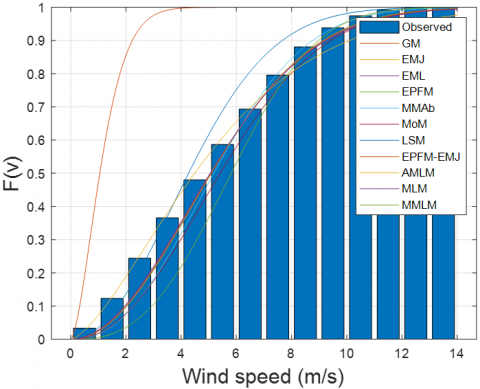
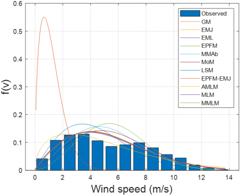
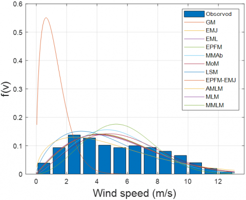
Figure 1 shows the modeled Weibull PDF and cumulative frequency distribution, plotted with the probability function $f(v)$ versus the mean wind speed, and the cumulative distribution $f(v)$ versus the mean wind speed. Figure 1 shows the results of the eleven methods, using one and 5 years of wind speed Reanalysis data of ERA5 of Barranquilla city in Colombia. The mean wind speed data as well as the standard deviation of the dataset of Barranquilla city are shown in Table 1.
Table 1. Mean wind speed and wind speed standard deviation
|
Year |
Mean wind speed (m/s) |
Standard deviation (m/s) |
|
2015 2016 2017 2018 2019 2020 |
6.0498 5.2830 4.9381 5.4223 5.3299 5.3245 |
2.9274 2.9785 2.7830 2.5991 2.6504 2.9180 |
The results of Figure 1 allow verifying how the curves Weibull PDF represents the wind speed distribution of Barranquilla city. In this sense, each of the eleven numerical methods considered in the analysis aims to match the histograms related to the observed data, which ease identifying which method achieves the best fit. Table 2 are listed the statistical results of the shape and scale parameters related to each method.
where, $\Gamma(\mathrm{t})$ is the gamma function defined as:
$\Gamma(\mathrm{t})=\int_{0}^{\infty} \exp (-x) x^{t-1} d x$
$\bar{v}$ is the mean of the wind speed.
$\bar{v}^{3}$ is the average wind speed cube.
$\overline{v^{3}}$ is the average of the cube of the wind speed.
$\sigma$ is the standard deviation.
$N$ is the number of observations.
$f\left(v_{i}\right)$ is the frequency of the wind speed measured in an Interval $i$.
$f(v \geq 0)$ is the probability that the wind speed is greater than or equal to zero.
4.1 Statistical
The modeled distributions plotted in Figure 1 pointed that the implicit methods that required numerical iterations, such as MoM, MLM, and MMLM, showed a better fit of the curve with the histogram, which evidenced that these models found successfully the shape parameter k and the scale parameter $C$ of the Weibull distribution. The statement is supported by the statistical results of RMSE, RRMSE, and $X^{2}$ (Table 3) which the implicit methods reported the best fitting values of k and c.
|
(a) Weibull distribution 2015-2020 |
(b) Cumulative frequency 2015-2020 |
|
(c) Weibull distribution 2015 |
(d) Weibull distribution 2016 |
|
(e) Weibull distribution 2017 |
(f) Weibull distribution 2018 |
|
(g) Weibull distribution 2019 |
(h) Weibull distribution 2020 |
Figure 1. Modeled Weibull distribution using several periods 2015-2020
According to the results of GM, it was observed that this method could not simulate the natural distribution of the wind speed (Figure 1), hence, the statistical results showed the highest values of RMSE, RRMSE, and $\chi^{2}$. These statistical results represent a low performance of the GM method when modeling the wind data distribution. It can be concluded that 10 of the 11 methods work well. The in-situ data distributions of wind speed plotted in Figure 1 (observed) reported wind speed values that agree with the wind characteristics of the study area reported by Rueda-Bayona et al. [17, 18], and the time series modeling performed by Rueda-Bayona et al. [19]. Because the wind speed data showed a slight bimodal distribution (Figure 1c, d, h), which could be associated with the local variability of the study area, it is recommended to develop Weibull PDF models capable to represent bimodalities in the data distribution. Orimoloye et al. [20] developed a bimodal model for representing wave data in the frequency domain, hence, the mathematical formulation of the equation developed in that study could be a reference for developing Weibull equations with two density peaks.
Table 2. Different Weibull estimation method
|
Method |
Mathematical expression |
|
Graphical methods (GM) |
$\ln \{\ln [1-F(v)]\}=k \ln (v)-k \ln (c)$ |
|
Moment’s methods (MoM) |
$\bar{v}=c \Gamma\left(1+\frac{1}{k}\right), \sigma=c\left[\Gamma\left(1+\frac{2}{k}\right)-\Gamma^{2}\left(1+\frac{1}{k}\right)\right]^{\frac{1}{2}}$ |
|
Energy pattern factor method (EPFM) |
$E_{p f}=\frac{\overline{v^{3}}}{\bar{v}^{3}}, k=1+\frac{3.69}{E_{p f}^{2}}, c=\frac{\bar{v}}{\Gamma\left(1+\frac{1}{k}\right)}$ |
|
Empirical method of Justus (EMJ) |
$k=\left(\frac{\sigma}{\bar{v}}\right)^{-1.086}, c=\frac{\bar{v}}{\Gamma\left(1+\frac{1}{k}\right)}$ |
|
Empirical method of Lysen (EML) |
$k=\left(\frac{\sigma}{\bar{v}}\right)^{-1.086}, c=\bar{v}\left(0.568+\frac{0.433}{\mathrm{k}}\right)^{-\frac{1}{k}}$ |
|
Maximum likelihood method (MLM) |
$k=\left[\frac{\sum_{i=1}^{N} v_{i}^{k} \ln v_{i}}{\sum_{i=1}^{N} v_{i}^{k}}-\frac{1}{N} \sum_{i=1}^{N} \ln v_{i}\right]^{-1}, c=\left[\frac{1}{N} \sum_{i=1}^{N} v_{i}^{k}\right]^{\frac{1}{k}}$ |
|
Modified Maximum likelihood method (MMLM) |
$k=\left[\frac{N \sum_{i=1}^{N} \ln v_{i} \ln \{-\ln [1-F(v)]\}-\sum_{i=1}^{N} \ln v_{i} \sum_{i=1}^{N} \ln \{-\ln [1-F(v)]\}}{\sum_{i=1}^{N} \ln v_{i}^{2}-\left(\sum_{i=1}^{N} \ln v_{i}\right)^{2}}\right]$ |
|
The last square method (LSM) |
$k=\left[\frac{N \sum_{i=1}^{N} \ln v_{i} \ln \{-\ln [1-F(v)]\}-\sum_{i=1}^{N} \ln v_{i} \sum_{i=1}^{N} \ln \{-\ln [1-F(v)]\}}{\sum_{i=1}^{N} \ln v_{i}^{2}-\left(\sum_{i=1}^{N} \ln v_{i}\right)^{2}}\right]$ |
|
Alternative maximum likelihood method (AMLM) |
$k=\frac{\pi}{\sqrt{6}}\left[\frac{N(N-1)}{N\left(\sum_{i=1}^{N} \ln v_{i}^{2}\right)-\left(\sum_{i=1}^{N} \ln v_{i}\right)^{2}}\right]^{\frac{1}{2}}, c=\left[\frac{1}{N} \sum_{i=1}^{N}\left(v_{i}\right)^{k}\right]^{\frac{1}{k}}$ |
|
The Mabchour method (MMAb) |
$k=1+(0.483(\bar{v}-2))^{0.51}, c=\frac{\bar{v}}{\Gamma\left(1+\frac{1}{k}\right)}$ |
|
Hybrid (EPFM-EMJ) |
$k=\frac{1}{2}\left(1+\frac{3.69}{E_{p f}^{2}}+\left(\frac{\sigma}{\bar{v}}\right)^{-1.086}\right), c=\frac{\bar{v}}{\Gamma\left(1+\frac{1}{k}\right)}$ |
Table 3. Wind speed statistical analysis of Barranquilla city
|
Year |
Numerical method |
Weibull parameters |
Statistical test |
|||
|
k |
c |
RMSE |
RRMSE (%) |
$\chi^{2}$ |
||
|
2015 |
GM EMJ EML EPFM MMab MoM LSM EPFM-EMJ AMLM MLM MMLM |
1.6670 2.1998 2.1998 2.2574 2.4080 2.1672 2.1395 2.2286 1.6624 2.1689 2.7520 |
1.3092 6.8311 6.8339 6.8301 6.8241 7.1019 5.7178 6.8307 6.5148 6.8172 8.6252 |
0.1355 0.0989 0.0989 0.1001 0.1030 0.0961 0.1069 0.0995 0.0899 0.0984 0.0932 |
2.2393 1.6351 1.6347 1.6541 1.7031 1.5880 1.7666 16446 1.4893 1.6268 1.5399 |
0.0194 0.0021 0.0020 0.0021 0.0021 0.0019 0.0028 0.0021 0.0022 0.0021 0.0013 |
|
2016 |
GM EMJ EML EPFM MMab MoM LSM EPFM-EMJ AMLM MLM MMLM |
1.4899 1.8633 1.8633 1.9064 2.2651 2.1662 1.9122 1.8848 1.4391 1.8230 2.6719 |
1.3518 5.9496 5.9536 5.9543 5.9643 6.3535 5.0128 5.9521 5.6508 5.9403 6.3514 |
0.1669 0.1024 0.1023 0.1087 0.1031 0.1025 0.1154 0.1027 0.0977 0.1018 0.1099 |
3.1598 1.9380 1.9371 1.9508 2.0584 1.9404 2.1847 1.9444 1.8490 1.9269 2.0803 |
0.0306 0.0031 0.0031 0.0031 0.0030 0.0026 0.0044 0.0031 0.0037 0.0031 0.0026 |
|
2017 |
GM EMJ EML EPFM MMab MoM LSM EPFM-EMJ AMLM MLM MMLM |
1.5453 1.8641 1.8641 1.8894 2.1954 2.1662 1.9832 1.8767 1.3956 1.8354 2.8280 |
1.3373 5.5612 5.5650 5.5639 5.5759 5.9383 4.7182 5.5626 5.2458 5.5585 3.3264 |
0.1729 0.1114 0.1113 0.1119 0.1176 0.1116 0.1270 0.1116 0.1047 0.1108 0.1113 |
3.5021 2.2556 2.2545 2.2651 2.3805 2.2605 2.5722 2.2603 2.1210 2.2446 2.5604 |
0.0321 0.0038 0.0038 0.0038 0.0038 0.0033 0.0054 0.0038 0.0046 0.0038 0.0038 |
|
2018 |
GM EMJ EML EPFM MMab MoM LSM EPFM-EMJ AMLM MLM MMLM |
1.6829 2.2224 2.2224 2.2502 2.2922 2.1662 1.8825 2.2363 1.5211 2.1960 3.0320 |
1.3059 6.1223 6.1247 6.1218 6.1208 6.3564 5.2687 6.1221 5.7468 6.1144 6.1268 |
0.1418 0.1139 0.119 0.1146 0.1156 0.1099 0.1140 0.1142 0.0986 0.1133 0.1319 |
2.6144 2.1005 2.1000 2.1129 2.1316 2.0269 2.1032 2.1067 1.8189 2.0903 2.4325 |
0.0213 0.0030 0.0030 0.0030 0.0030 0.0027 0.0037 0.0030 0.0030 0.0030 0.0035 |
|
2019 |
GM EMJ EML EPFM MMab MoM LSM EPFM-EMJ AMLM MLM MMLM |
1.6431 2.1355 2.1355 2.1841 2.2742 2.1662 1.8381 2.1598 1.4852 2.1033 2.7824 |
1.3143 6.0183 6.0210 6.0183 6.0170 6.2825 5.0827 6.0184 5.6524 6.0082 6.9059 |
0.1555 0.1109 0.1108 0.1120 0.1140 0.1087 0.1137 0.1114 0.0984 0.1103 0.1137 |
2.9172 2.0803 2.0797 2.1008 2.1387 2.0388 2.1337 2.0905 1.8463 2.0686 2.1340 |
0.0252 0.0030 0.0030 0.0030 0.0031 0.0028 0.0040 0.0030 0.0033 0.0030 0.0025 |
|
2020 |
GM EMJ EML EPFM MMab MoM LSM EPFM-EMJ AMLM MLM MMLM |
1.4908 1.9216 1.9216 1.9681 2.2732 2.1662 1.6677 1.9448 1.4543 1.8819 2.7518 |
1.3515 6.0025 6.0063 6.0061 6.0110 6.3733 5.1326 6.0044 5.6876 5.9929 6.2075 |
0.1578 0.1033 0.1033 0.1041 0.1031 0.1091 0.1087 0.1037 0.0975 0.1028 0.1140 |
2.9640 1.9409 1.9400 1.9553 2.0495 1.9364 2.0406 1.9481 1.8309 1.9297 2.1403 |
0.0280 0.0030 0.0030 0.0030 0.0030 0.0026 0.0042 0.0030 0.0035 0.0030 0.0028 |
4.2 Analysis of the values of the parameters k and c
The calculated Weibull parameters can be observed in Table 3, where the parameter $k$ showed values from 2.1 to 2.7. The parameter c showed values nearby to 6, where the GM method showed the lowest values close to 1 and the MMLM method pointed to the highest value equal to 8.6252f for 2015. The calculus of the parameter k for the numerical iteration methods MoM, MLM, and MMLM were performed through MATLAB programming. Then, were required k data vectors limited by k, $0.0001 \leq k \leq 5$ with increments (delta) of 0.0001 per iteration. Because the delta required for the numerical interactions increases the computational time for solving the implicit methods, this study performed and performance test of the numerical methods to identify the proper delta value of each method. As a result, the delta (0.0001) was set for the computations. Considering that the c parameter is in the function of the k parameter, its calculation was explicitly and easy to handle for the MMLM, MLM, and AMLM methods. For finding the Weibull parameters of the MoM method, it was required to set anonymous MATLAB functions using seed values of k and c as initial conditions.
The calculation of the shape and scale parameters for the Weibull function was determined. Eleven methods found in the literature were solved using hourly wind speed data obtained from the ERA5 database. The results revealed that GM could not simulate properly the wind speed data distribution because Table 2 can see a low accuracy compared with other methods. On the contrary, the numerical iteration methods MoM, ALMM, MLM, and MMLM not only could fit into the wind speed distribution but also had the best performance when simulating the wind data distribution considering the results of RMSE, RRMSE, and with numbers less than 0.09, 0.1, 1.7 and 2.2, and values close to zero respectively, showing excellent performance and high accuracy. The MLM and MMLM methods showed a high computational consumption, because of k values vector the larger is its size the better the fit results are. However, to optimize the calculation process, we recommend controlling the k input vector to avoid out of memory when running the programming code. Finally, this study concluded that the best method for representing wind speed data distributions through the Weibull PDF model were MLM, MMLM, and MoM, and as future research is recommended to develop new methods when wind data have bimodal distributions.
[1] Carneiro, T.C., Melo, S.P., Carvalho, P.C., Braga, A.P.D.S. (2016). Particle swarm optimization method for estimation of Weibull parameters: A case study for the Brazilian northeast region. Renewable Energy, 86: 751-759. https://doi.org/10.1016/j.renene.2015.08.060
[2] Pryor, S.C., Barthelmie, R.J., Bukovsky, M.S., Leung, L.R., Sakaguchi, K. (2020). Climate change impacts on wind power generation. Nature Reviews Earth & Environment, 1(12): 627-643. https://doi.org/10.1038/s43017-020-0101-7
[3] Haque, A.U., Mandal, P., Meng, J., Kaye, M.E., Chang, L. (2012). A new strategy for wind speed forecasting using hybrid intelligent models. In 2012 25th IEEE Canadian Conference on Electrical and Computer Engineering (CCECE), Montreal, QC, Canada, pp. 1-4. https://doi.org/10.1109/CCECE.2012.6334847
[4] Mohammadi, K., Alavi, O., Mostafaeipour, A., Goudarzi, N., Jalilvand, M. (2016). Assessing different parameters estimation methods of Weibull distribution to compute wind power density. Energy Conversion and Management, 108: 322-335. https://doi.org/10.1016/j.enconman.2015.11.015
[5] Wais, P. (2017). A review of Weibull functions in wind sector. Renewable and Sustainable Energy Reviews, 70: 1099-1107. https://doi.org/10.1016/j.rser.2016.12.014
[6] Murthy, K.S.R., Rahi, O.P. (2017). A comprehensive review of wind resource assessment. Renewable and Sustainable Energy Reviews, 72: 1320-1342. https://doi.org/10.1016/j.rser.2016.10.038
[7] Guenoukpati, A., Salami, A.A., Kodjo, M.K., Napo, K. (2020). Estimating Weibull parameters for wind energy applications using seven numerical methods: Case studies of three coastal sites in West Africa. International Journal of Renewable Energy Development, 9(2): 217-226, https://doi.org/10.14710/ijred.9.2.217-226
[8] Masseran, N. (2015). Evaluating wind power density models and their statistical properties. Energy, 84: 533-541. https://doi.org/10.1016/j.energy.2015.03.018
[9] Chang, T.P. (2011). Performance comparison of six numerical methods in estimating Weibull parameters for wind energy application. Applied Energy, 88(1): 272-282. https://doi.org/10.1016/j.apenergy.2010.06.018
[10] Rocha, C. (2012). Comparison of seven numerical methods for determining Weibull parameters for wind energy generation in the northeast region of Brazil. Appl. Energy, 89: 395-400. https://doi.org/10.1016/j.apenergy.2011.08.003
[11] Arslan, T., Bulut, Y.M., Yavuz, A.A. (2014). Comparative study of numerical methods for determining Weibull parameters for wind energy potential. Renewable and Sustainable Energy Reviews, 40: 820-825. https://doi.org/10.1016/j.rser.2014.08.009
[12] Kapen, P.T., Gouajio, M.J., Yemélé, D. (2020). Analysis and efficient comparison of ten numerical methods in estimating Weibull parameters for wind energy potential: Application to the city of Bafoussam, Cameroon. Renewable Energy, 159: 1188-1198. https://doi.org/10.1016/j.renene.2020.05.185
[13] Bilir, L., Imir, M., Devrim, Y., Albostan, A. (2015). Seasonal and yearly wind speed distribution and wind power density analysis based on Weibull distribution function. International Journal of Hydrogen Energy, 40(44): 15301-15310. https://doi.org/10.1016/j.ijhydene.2015.04.140
[14] Usta, I. (2016). An innovative estimation method regarding Weibull parameters for wind energy applications. Energy, 106: 301-314. https://doi.org/10.1016/j.energy.2016.03.068
[15] Chaurasiya, P.K., Ahmed, S., Warudkar, V. (2018). Comparative analysis of Weibull parameters for wind data measured from met-mast and remote sensing techniques. Renewable Energy, 115: 1153-1165. 10.1016/j.renene.2017.08.014
[16] Tizgui, I., El Guezar, F., Bouzahir, H., Benaid, B. (2017). Comparison of methods in estimating Weibull parameters for wind energy applications. International Journal of Energy Sector, 11(4): 650-663. https://doi.org/10.1108/IJESM-06-2017-0002
[17] Rueda-Bayona, J.G., Elles Pérez, C.J., Sánchez Cotte, E.H., González Ariza, Á.L., Rivillas Ospina, G.D. (2016). Identificación de patrones de variabilidad climática a partir de análisis de componentes principales, Fourier y clúster k-medias. Tecnura, 20(50): 55-68. https://doi.org/10.14483/udistrital.jour.tecnura.2016.4.a04
[18] Rueda-Bayona, J.G. (2017). Identificación de la influencia de las variaciones convectivas en la generación de cargas transitorias y su efecto hidromecánico en las estructuras Offshore. PhD Thesis, Universidad del Norte, Barranquilla, Colombia.
[19] Rueda-Bayona, J.G., Cabello Eras, J.J., Sagastume, A. (2021). Modeling wind speed with a long-term horizon and high-time interval with a hybrid Fourier-neural network model. Mathematical Modelling of Engineering Problems, 8(3): 431-440. https://doi.org/10.18280/mmep.080313
[20] Orimoloye, S., Horrillo-Caraballo, J., Karunarathna, H., Reeve, D.E. (2021). Wave overtopping of smooth impermeable seawalls under unidirectional bimodal sea conditions. Coastal Engineering, 165: 103792. https://doi.org/10.1016/j.coastaleng.2020.103792