Mallinath Dhange | Gurunath Sankad* | Umesh Bhujakkanavar
© 2021 IIETA. This article is published by IIETA and is licensed under the CC BY 4.0 license (http://creativecommons.org/licenses/by/4.0/).
OPEN ACCESS
In the present manuscript, a mathematical model of steady and incompressible Casson fluid in a non-uniform tube having many stenoses in the presence of a force field is analyzed. Using mild stenosis approximation and appropriate boundary conditions, analytical expressions for velocity, pressure drop, impedance, and wall share stress have been computed due to their importance in the rheology of blood. The Casson fluid is used to depict the behavior of blood flow. The effects of different physical constraints on resistance to the flow and wall shear stress of the fluid are examined. The study ascertains that resistance to the flow and wall shear stress is maximum at duck of stenosis. It is also explored that an increase in the size of the stenosis in the artery affects the normal flow of the blood through vessels in the heart, body, and brain and this may lead to major cardiac disease problems like stroke, heart attack, etc.
multiple stenoses, Casson fluid, force field, impedance, wall shear stress
The term stenosis indicates the narrowing of the artery because of the development of the arteriosclerotic deposition or different sorts of anomalous tissue development. As the development ventures into the lumen of the artery, blood flow is impeded. The impediment may harm the inner cells of the wall and may prompt further development of the stenosis. In this way, there is a coupling between the development of stenosis and the flow of blood in the artery since it influences the other. The advancement of stenosis in an artery can have genuine outcomes and can disturb the typical working of the circulatory system. Specifically, it might prompt: increased resistance to flow with the possible serious decrease in blood flow, increased risk of complete occlusion, abnormal cell development in the region of the stenosis, which builds the intensity of the stenosis, and tissue harm prompting post stenosis dilatation.
The examination of blood flow through vessels with stenosis is one of the principal territories of research since more than 30% of all deaths because by circularity issues and these circularity issues can have results, for example, pain in the chest and decreasing bloodstream to the brain. Cardiovascular breakdown, which builds the risk of death. The main reason for circularity disorders is stenosis. The stenotic artery, which diminishes the bloodstream, is a typical cardiovascular disorder. Stenosis can alter the normal functioning of the heart system. It also increases the impedance to blood flows, resulting in increased blood pressure and tissue damage leading to subsequent stenotic dilation. Stenosis was first studied by Young [1]. Azuma and Fukushima [2] investigated the disturbances of blood flow through stenotic blood vessels. Axisymmetric and nonsymmetric models having different diameter ratios of constriction were used in the experiments. MacDonald [3] revealed the technique for steady flow through the mild axisymmetric arterial stenoses model. The steady flow of an incompressible fluid through an axisymmetric converging-diverging tube has been studied both theoretically (Part I) and experimentally (Part II) by Forrester and Young [4]. They established the mathematical model for mild stenosis and an approximate solution for flow through a converging-diverging tube is obtained. Shukla et al. [5] studied the effects of stenosis on non-Newtonian flow through an artery with mild stenosis. Later, numerous researchers have considered the flow features of blood in a tube with mild constriction by taking blood as Newtonian or non- Newtonian fluids in diverse situations [5-9].
The examination of the non-Newtonian nature of blood flow has been of most significance to scientists lately because of their application in exploring the conduct of blood on small arteries. Most of the works done in the literature are carried out by taking Newtonian fluid, micropolar, Herschel-Bulkley, and Jeffrey models. This approach neglects to clarify the physiological conduct of the bloodstream in supply routes because of the presence of yield stress. Even though Herschel-Bulkley flow contains yield stress constraint, it is found that at low shear rates Casson model fits the blood flow better than that of Herschel-Bulkley fluid (see Blair [10]). Chaturani and Samy [11] explored the applications to the blood flow through the pulsatile flow of Casson’s fluid with stenosed arteries. Bali and Awasthi [12] studied the impacts of magnetic field on Casson fluid model for various stenosed artery. In this way, various researchers did the investigation of Casson fluid under different physiological situations in recent times [13, 14].
It is known that many ducts in physiological systems are not horizontal but have some inclination to the axis. Maruti Prasad and Radhakrishnamacharya [15] explored the blood flow through an artery having multiple stenoses with a non-uniform cross-section. The effects of an axially symmetric mild stenosis on the flow of blood when blood is represented by a couple stress fluid model have been studied by Srivastava [16]. Ponalagusamy [17] studied the mathematical model for a steady flow of blood through tapered stenosed arteries with a peripheral plasma layer near the wall. The model consists of a core region of suspension of all the erythrocytes assumed to be a couple stress fluid and a peripheral layer of plasma as a Newtonian fluid. Varma and Parihar [18] and Sharma et al. [19] studied the impact of an external magnetic field applied consistently in a multistage stenosis artery in the central region and presumed that the impact of the yield stress and stenosis is to decrease the shear stress of the wall and the speed of the flow within the sight of the magnetic field. Lately, numerous specialists have considered the attributes of blood flow through the artery within the sight of stenosis [20-35].
In the literature review, it is observed that many investigators have worked on the blood flow through stenosed arteries with various fluids and geometries. However, no investigation has demonstrated the effects of multi-stage stenoses and a Casson fluid with mild stenosis condition. With the above inspiration, an attempt has been made to examine the effects of multi-stage stenosis on an incompressible Casson fluid through a non-uniform inclined tube in the presence of a force field. The investigation is done analytically. The outcomes of the present study are analyzed through graphs. The physical and mathematical models are described in detail in section 2. Thereafter, section 3 is for the discussion of the obtained outcomes.
The term stenosis indicates the narrowing of the artery because of the development of the arteriosclerotic deposition or different sorts of anomalous tissue development. As the development Consider the flow of an incompressible Casson fluid through an inclined axisymmetric tube of the non-uniform cross-section with multiple stenoses. The cylindrical polar coordinate system (z, r) is chosen so that the z-axis coincides with the centreline of the tube. The stenosis is supposed to be mild and develop in an axially symmetric manner. The geometry of the wall is as shown in Figure 1.
Figure 1. Schematic diagram of the tube with stenosis
The equation relating the geometry of the wall is (Maruti Prasad and Radhakrishnamacharya [15]).
$h(z)=\left\{\begin{array}{cc}R_{0} & : 0 \leq z \leq d_{1} \\ R_{0}-\frac{\delta_{1}}{2}\left(1+\cos \frac{2 \pi}{L_{1}}\left\langle z-d_{1}-\frac{L_{1}}{2}\right\rangle\right) & : d_{1} \leq z \leq d_{1}+L_{1} \\ R_{0} & : d_{1}+L_{1} \leq z \leq B_{1}-\frac{L_{2}}{2} \\ R_{0}-\frac{\delta_{1}}{2}\left(1+\cos \frac{2 \pi}{L_{2}}\left\langle z-B_{1}\right\rangle\right) & : B_{1}-\frac{L_{2}}{2} \leq z \leq B_{1} \\ R^{*}(z)-\frac{\delta_{2}}{2}\left(1+\cos \frac{2 \pi}{L_{2}}\left\langle z-B_{1}\right\rangle\right) & : B_{1} \leq z \leq B_{1}+\frac{L_{2}}{2} \\ R^{*}(z) & : B_{1}+\frac{L_{2}}{2} \leq z \leq B,\end{array}\right.$ (1)
where, B- the length of the channel, $L_{1}, L_{2}-$ the lengths, and $\delta_{1}, \delta_{2}-$ the maximum heights of the primary and secondary stenosis respectively.
Referring to ref. [15], the limitations for mild stenosis are taken into account as:
$\min \left(R_{0}, R_{\text {out }}\right) \gg \delta_{1}, \delta_{2}$, and $L_{1}, L_{2} \gg \delta_{1}, \delta_{2}$,
where, $R(z)=R_{\text {out }}$ at $z=B$.
The governing equation of the flow for the present issue is given as:
$\frac{1}{r} \frac{\partial}{\partial r}\left(r \tau_{r z}\right)=-\frac{1}{\mu} \frac{\partial p}{\partial z}+\rho g \sin \alpha-M^{\prime} \mu_{0} \frac{\partial H^{\prime}}{\partial z}$, (2)
where,
$\sqrt{\tau_{r z}}=\left\{\begin{array}{cl}\sqrt{\mu} \sqrt{-\frac{\partial u}{\partial r}}+\sqrt{\tau_{0}} & : \tau \geq \tau_{0} \\ 0 & : \tau \leq \tau_{0}.\end{array}\right.$ (3)
Here, $\mu_{0}-$ the magnetic permeability, M'-magnetization, $H^{\prime}-$ magnetic field intensity, $\tau_{r z}$- the shear stress, $\mu-$ blood viscosity, $\tau_{0}-$ yield stress, $(r, z)-$ respectively radial and axial coordinates.
Considering the forces in the plug region, it yields as:
$2 \pi r_{0} B \tau_{0}=P \pi r_{0}^{2} B \quad \therefore \tau_{0}=\frac{P r_{0}}{2}$,
where, $P=\frac{\partial p}{\partial z}$ (4)
The conditions of the boundary are specified as:
$\tau_{r z}$ is finite $\quad$ at $r=0$ (5)
$u=0 \quad$ at $\quad r=h$ (6)
Taking the restriction for mild stenosis and solving (2) under the boundary conditions (5) and (6), the velocity is yield as:
$u=\frac{(P+f+K)}{2 \mu}\left[\frac{4}{3} r_{0}^{\frac{1}{2}}\left(r^{\frac{3}{2}}-h^{\frac{3}{2}}\right)-\frac{1}{2}\left(r^{2}-h^{2}\right)-r_{0}(r-h)\right]$ (7)
Substituting $r=r_{0}$ in the above equation, we get the plug velocity as:
$u_{p}=\frac{(P+f+K)}{2 \mu}\left[-\frac{1}{6} r_{0}^{2}-\frac{4}{3} r_{0}^{\frac{1}{2}} h^{\frac{3}{2}}+\frac{1}{2} h^{2}+h r_{0}\right]$ (8)
where, $f=\frac{\sin \alpha}{F}, K=\frac{\mu_{0} M H_{0}}{\rho U_{0}^{2}}, F=\frac{\mu u^{\frac{1}{2}}}{\rho g R_{0}^{\frac{3}{2}}}$.
The flux Q of the fluid is given as:
$Q=2 \int_{0}^{r_{0}} u_{p} r d r+2 \int_{r_{0}}^{h} u r d r$ (9)
$\therefore Q=\frac{(P+f+K)}{\mu}\left[-\frac{1}{168} r_{0}^{4}-\frac{2}{7} r_{0}^{\frac{1}{2}} h^{\frac{7}{2}}+\frac{1}{8} h^{4}+\frac{1}{6} h^{3} r_{0}\right]$ (10)
The non-dimensional quantities are specified as:
$r^{\prime}=\frac{r}{R_{0}}, r_{0}^{\prime}=\frac{r_{0}}{R_{0}}, \delta_{1}^{\prime}=\frac{\delta_{1}}{R_{0}}, \delta_{2}^{\prime}=\frac{\delta_{2}}{R_{0}}, H=\frac{h}{R_{0}},$
$Z^{\prime}=\frac{Z}{B}, L_{1}^{\prime}=\frac{L_{1}}{B}, L_{2}^{\prime}=\frac{L_{2}}{B}, B_{1}^{\prime}=\frac{B_{1}}{B},$
$H^{\prime}=\frac{M}{H_{0}}, u=\frac{u^{\prime}}{U_{0}}, d_{1}^{\prime}=\frac{d_{1}}{B}, d_{2}^{\prime}=\frac{d_{2}}{B},$
$Q^{\prime}=\frac{Q}{U_{0} R_{0}^{2}}, R^{*}\left(Z^{\prime}\right)=\frac{R^{*}(z)}{R_{0}}, p^{\prime}=\frac{p}{\frac{\mu U_{0} B}{R_{0}^{2}}},$
$r_{0}^{\prime}=\frac{r_{0}}{R_{0}}, r^{\prime}=\frac{r}{R_{0}}$. (11)
From Eq. (10), Eq. (11) yields as:
$Q=(P+f+K)\left[-\frac{1}{168} r_{0}^{4}-\frac{2}{7} r_{0}^{\frac{1}{2}} H^{\frac{7}{2}}+\frac{1}{8} H^{4}+\frac{1}{6} H^{3} r_{0}\right]$ (12)
Eq. (12) can be expressed as:
$\frac{\partial p}{\partial z}=-\frac{Q}{\left[-\frac{1}{168} r_{0}^{4}-\frac{2}{7} r_{0}^{\frac{1}{2}} H^{\frac{7}{2}}+\frac{1}{8} H^{4}+\frac{1}{6} H^{3} r_{0}\right.}+f+K$ (13)
The primitive of the Eq. (13) gives the pressure difference $\Delta p$ along the total length of the channel as:
$\Delta p=\int_{0}^{1} \frac{\partial p}{\partial z} d z=\int_{0}^{1}\left\{\frac{-Q}{\left[\begin{array}{c}-\frac{1}{168} r_{0}^{4}-\frac{2}{7} r_{0}^{\frac{1}{2}} H^{\frac{7}{2}} \\ +\frac{1}{8} H^{4}+\frac{1}{6} H^{3} r_{0}\end{array}\right]}+f+K\right\} d z$ (14)
The resistance to flow is defined as:
$\lambda=\frac{\Delta p}{Q}$ (15)
From Eq. (14) and (15), we get,
$\lambda=\frac{1}{Q} \int_{0}^{1}\left\{\frac{-Q}{\left[-\frac{1}{168} r_{0}^{4}-\frac{2}{7} r_{0}^{\frac{1}{2}} H^{\frac{7}{2}}+\frac{1}{8} H^{4}+\frac{1}{6} H^{3} r_{0}\right]}+f+K\right\} d z$ (16)
In the absence of stenosis (H=1), the pressure drop is obtained as:
$(\Delta p)_{n}=\int_{0}^{1}\left\{\frac{-Q}{\left[-\frac{1}{168} r_{0}^{4}-\frac{2}{7} r_{0}^{\frac{1}{2}}+\frac{1}{8}+\frac{1}{6} r_{0}\right]}+f+K\right\} d z$ (17)
In the absence of stenosis, resistance to the flow is defined as:
$\lambda_{n}=\frac{(\Delta p)_{n}}{Q}$ (18)
From Eq. (17) and (18), we acquire,
$\lambda_{n}=\frac{1}{Q} \int_{0}^{1}\left\{\frac{-Q}{\left[-\frac{1}{168} r_{0}^{4}-\frac{2}{7} r_{0}^{\frac{1}{2}}+\frac{1}{8}+\frac{1}{6} r_{0}\right]}+f+K\right\} d z$ (19)
The normalized resistance to the flow is specified as:
$\bar{\lambda}=\frac{\lambda}{\lambda_{n}}$ (20)
The shear stress acting on the wall of the channel is given by:
$\tau_{w}=-\left.\mu \frac{\partial u}{\partial r}\right|_{r=h}$ (21)
Applying dimensional quantities (11) to Eq. (21), it gives:
$\tau_{w}^{\prime}=\frac{\tau_{w}}{\left[\frac{\mu U}{R_{0}}\right]}$ (22)
Eq. (22) reduces to:
$\tau_{w}^{\prime}=-\frac{\partial u^{\prime}}{\partial r^{\prime}}$ (23)
Utilizing Eq. (7) in non-dimensional form and Eq. (13) in Eq. (23), we get:
$\tau_{w}=\frac{-Q}{2}\left\{\frac{2 r_{0}^{\frac{1}{2}} H^{\frac{1}{2}}-H-r_{0}}{\frac{1}{168} r_{0}^{4}+\frac{2}{7} r_{0}^{\frac{1}{2}} H^{\frac{7}{2}}-\frac{1}{8} H^{4}-\frac{1}{6} H^{3} r_{0}}\right\}+f+K$ (24)
In the absence of stenosis (H=1), the shear stress at the wall is computed from Eq. (24) as:
$\left(\tau_{w}\right)_{n}=\frac{-Q}{2}\left\{\frac{2 r_{0}^{\frac{1}{2}}-1-r_{0}}{\frac{1}{168} r_{0}^{4}+\frac{2}{7} r_{0}^{\frac{1}{2}}-\frac{1}{8}-\frac{1}{6} H^{3} r_{0}}\right\}+f+K$ (25)
The normalized shear stress at the wall is specified as:
$\bar{\tau}_{w}=\frac{\tau_{w}}{\left(\tau_{w}\right)_{n}}$ (26)
The resistance to the flow and wall shear stress are two key characteristics in the study of blood flow through a stenosed artery. Analytical solutions for flow resistance $(\bar{\lambda})$ and wall shear stress $\left(\bar{\tau}_{w}\right)$ are indicated by Eq. (20) and (26). The special effects of several constraints on flow resistance $(\bar{\lambda})$ and wall shear stress $\left(\bar{\tau}_{w}\right)$ are computed numerically by using MATHEMATICA and results are presented through graphs.
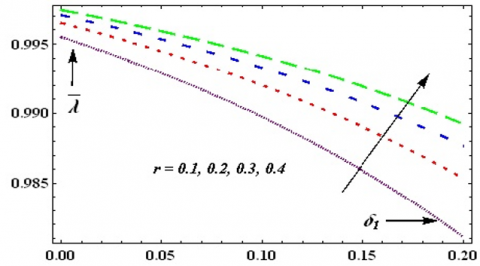
Figures 2-25 illustrate the effects of impedance and wall shear stress on various constraints with stenosis heights ($\left.\delta_{1}, \delta_{2}\right)$. It is noticed that impedance $(\bar{\lambda})$ ascends and wall shear stress $\left(\bar{\tau}_{w}\right)$ descends with the radial distance of the plug region (Figures 2, 4, 14, and 16 when F=0.1 and Figures 3, 5, 15, and 17 when F=0.3), i.e. the impedance increases and shear stress of wall decreases with a non-Newtonian character of the Casson liquid. Furthermore, an impedance of the flow $(\bar{\lambda})$ increases with growth in magnetic force field constraint (M) (see Figures 6, 8 when F=0.1 and Figures 7, 9 when F=0.3) and angle of proclivity (α) when F=0.1 (Figures 10 and 12) and F=0.3 (Figures 11 and 13). These results match with the earlier outcomes of Shukla et al. [5], Maruti Prasad and Radhakrishnamacharya [15], and Verma and Parihar [18].
Figures 14-25 illustrate the impacts of wall shear stress $\left(\bar{\tau}_{w}\right)$ with stenosis heights ($\left.\delta_{1}, \delta_{2}\right)$. It is observed that wall shear stress $\left(\bar{\tau}_{w}\right)$ also increases with magnetic forced field constraint $(M)$ and angle of proclivity $(\alpha)$ (respectively Figures 18, 20, 22, and 24 when $F=0.1$ and Figures 19, 21, 23, and 25 when F=0.3). These outputs are linked with the past outcomes of Young [1], MarutiPrasad, and Radhakrishnamacharya [15]. The behavior of impedance and wall shear stress on both heights ($\left.\delta_{1}, \delta_{2}\right)$ of stenosis are illustrated in Figures 26-29. It is also seen that $\bar{\lambda}$ and $\bar{\tau}_{w}$ acting over both heights ($\left.\delta_{1}, \delta_{2}\right)$ of stenosis. These outputs are linked with the past outcomes of Young [1], Shukla et al. [5], Maruti Prasad, and Radhakrishnamacharya [15].
Figure 2. Sketch of $\delta_{1}$ & r on $\bar{\lambda}$ with $d_{1}=0.2, d_{2}=0.6, L_{1}=L_{2}=0.2, q=0.1, F=0.1, \alpha=\pi / 6, M=0.5$
Figure 3. Sketch of $\delta_{1}$ & $\bar{\alpha}, r$ on $\bar{\lambda}$ with $d_{1}=0.2, d_{2}=0.6, L_{1}=L_{2}=0.2, q=0.1, F=0.3, \alpha=\pi / 6, M=0.5$
Figure 4. Sketch of $\delta_{2}$ & r on $\bar{\lambda}$ with $d_{1}=0.2, d_{2}=0.6, L_{1}=L_{2}=0.2, q=0.1, F=0.1, \alpha=\pi / 6, M=0.5$
Figure 5. Sketch of $\delta_{2} \& r$ on $\bar{\lambda}$ with $d_{1}=0.2, d_{2}=0.6, L_{1}=L_{2}=0.2, q=0.1, F=0.3, \alpha=\pi / 6, M=0.5$
Figure 6. Sketch of $\delta_{1} \& M$ on $\bar{\lambda}$ with $d_{1}=0.2, d_{2}=0.6, L_{1}=L_{2}=0.2, q=0.1, F=0.1, r=0.2, \alpha=\pi / 6$
Figure 7. Sketch of $\delta_{1} \& M$ on $\bar{\lambda}$ with $d_{1}=0.2, d_{2}=0.6, L_{1}=L_{2}=0.2, q=0.1, F=0.3, r=0.2, \alpha=\pi / 6$
Figure 8. Sketch of $\delta_{2} \& M$ on $\bar{\lambda}$ with $d_{1}=0.2, d_{2}=0.6, L_{1}=L_{2}=0.2, q=0.1, F=0.1, r=0.2, \alpha=\pi / 6$
Figure 9. Sketch of $\delta_{2} \& M$ on $\bar{\lambda}$ with $d_{1}=0.2, d_{2}=0.6, L_{1}=L_{2}=0.2, q=0.1, F=0.3, r=0.2, \alpha=\pi / 6$
Figure 10. Sketch of $\delta_{1} \& \alpha$ on $\bar{\lambda}$ with $d_{1}=0.2, d_{2}=0.6, L_{1}=L_{2}=0.2, q=0.1, F=0.1, r=0.2, M=0.5$
Figure 11. Sketch of $\delta_{1} \& \alpha$ on $\bar{\lambda}$ with $d_{1}=0.2, d_{2}=0.6, L_{1}=L_{2}=0.2, q=0.1, F=0.3, r=0.2, M=0.5$
Figure 12. Sketch of $\delta_{2} \& \alpha$ on $\bar{\lambda}$ with $d_{1}=0.2, d_{2}=0.6, L_{1}=L_{2}=0.2, q=0.1, F=0.1, r=0.2, M=0.5$
Figure 13. Sketch of $\delta_{2} \& \alpha$ on $\bar{\lambda}$ with $d_{1}=0.2, d_{2}=0.6, L_{1}=L_{2}=0.2, q=0.1, F=0.3, r=0.2, M=0.5$
Figure 14. Sketch of $\delta_{1} \& r$ on $\bar{\tau}_{w}$ with $d_{1}=0.2, d_{2}=$ $0.6, L_{1}=L_{2}=0.2, q=0.1, F=0.1, M=0.5, \alpha=\pi / 6$
Figure 15. Sketch of $\delta_{1} \& r$ on $\bar{\tau}_{w}$ with $d_{1}=0.2, d_{2}=$ 0.6, $L_{1}=L_{2}=0.2, q=0.1, F=0.3, M=0.5, \alpha=\pi / 6$
Figure 16. Sketch of $\delta_{2} \& r$ on $\bar{\tau}_{w}$ with $d_{1}=0.2, d_{2}=$0.6, L_{1}=L_{2}=0.2, q=0.1, F=0.1, \alpha=\pi / 6, M=0.5$
Figure 17. Sketch of $\delta_{2} \& r$ on $\bar{\tau}_{w}$ with $d_{1}=0.2, d_{2}=0.6, L_{1}=L_{2}=0.2, q=0.1, F=0.3,, \alpha=\pi / 6, M=0.5$
Figure 18. Sketch of $\delta_{1} \& M$ on $\bar{\tau}_{w}$ with $d_{1}=0.2, d_{2}=0.6, L_{1}=L_{2}=0.2, q=0.1, F=0.1, r=0.2, \alpha=\pi / 6$
Figure 19. Sketch of $\delta_{1} \& M$ on $\bar{\tau}_{w}$ with $d_{1}=0.2, d_{2}=0.6, L_{1}=L_{2}=0.2, q=0.1, F=0.3, r=0.2, \alpha=\pi / 6$
Figure 20. Sketch of $\delta_{2} \& M$ on $\bar{\tau}_{w}$ with $d_{1}=0.2, d_{2}=0.6, L_{1}=L_{2}=0.2, q=0.1, F=0.1, r=0.2, \alpha=\pi / 6$
Figure 21. Sketch of $\delta_{2} \& M$ on $\bar{\tau}_{w}$ with $d_{1}=0.2, d_{2}=0.6, L_{1}=L_{2}=0.2, q=0.1, F=0.3, r=0.2, \alpha=\pi / 6$
Figure 22. Sketch of $\delta_{1} \& \alpha$ on $\bar{\tau}_{w}$ with $d_{1}=0.2, d_{2}=0.6, L_{1}=L_{2}=0.2, q=0.1, F=0.3,, r=0.2, M=0.5$
Figure 23. Sketch of $\delta_{1} \& \alpha$ on $\bar{\tau}_{w}$ with $d_{1}=0.2, d_{2}=0.6, L_{1}=L_{2}=0.2, q=0.1, F=0.3,, r=0.2, M=0.5$
Figure 24. Sketch of $\delta_{2} \& \alpha$ on $\bar{\tau}_{w}$ with $d_{1}=0.2, d_{2}=0.6, L_{1}=L_{2}=0.2, q=0.1, F=0.3, r=0.2, M=0.5$
Figure 25. Sketch of $\delta_{2} \& \alpha$ on $\bar{\tau}_{w}$ with $d_{1}=0.2, d_{2}=0.6, L_{1}=L_{2}=0.2, q=0.1, F=0.3,, r=0.2, M=0.5$
Figure 26. Sketch of $\delta_{1} \& \delta_{2}$ on $\bar{\lambda}$ with $d_{1}=0.2, d_{2}=0.6, L_{1}=L_{2}=0.2, q=0.1, F=0.3, r=0.2, M=0.5, \alpha=\pi / 6$
Figure 27. Sketch of $\delta_{2} \& \delta_{1}$ on $\bar{\lambda}$ with $d_{1}=0.2, d_{2}=0.6, L_{1}=L_{2}=0.2, q=0.1, F=0.3,, r=0.2, M=0.5, \alpha=\pi / 6$
Figure 28. Sketch of $\delta_{1} \& \delta_{2}$ on $\bar{\tau}_{w}$ with $d_{1}=0.2, d_{2}=0.6, L_{1}=L_{2}=0.2, q=0.1, F=0.3,, r=0.2, M=0.5, \alpha=\pi / 6$
Figure 29. Sketch of $\delta_{2} \& \delta_{1}$ on $\bar{\tau}_{w}$ with $d_{1}=0.2, d_{2}=0.6, L_{1}=L_{2}=0.2, q=0.1, F=0.3,, r=0.2, M=0.5, \alpha=\pi / 6$
In the present study, we have theoretically discussed the steady and incompressible Casson fluid flow through an inclined non-uniform tube with multiple stenoses under the influence of the force field. The concluding remarks are:
The impedance of the flow $(\bar{\lambda})$ increases and the wall shear stress $\left(\bar{\tau}_{w}\right)$ decreases as an increase in the radial distance of the plug flow region (r).
An increase in the non-Newtonian character of the Casson fluid the impedance of the flow $(\bar{\lambda})$ ascends and wall shear stress $\left(\bar{\tau}_{w}\right)$ descends.
The impedance of the flow $(\bar{\lambda})$ increases with growth in magnetic force field constraint (M) and angle of proclivity (α).
The wall shear stress $\left(\bar{\tau}_{w}\right)$ also increases with magnetic forced field constraint (M) and angle of proclivity (α).
An increase in heights ($\left.\delta_{1}, \delta_{2}\right)$ of the stenosis decelerates the wall shear stress and resistance to the flow.
|
B |
Length of the channel |
|
$L_{1}$ |
Length of primary stenosis |
|
$L_{2}$ |
Length of secondary stenosis |
|
$\delta_{1}$ |
Maximum height of primary stenosis |
|
$\delta_{2}$ |
Maximum height of secondary stenosis |
|
r |
Radial coordinate |
|
α |
Angle of proclivity |
|
$\bar{\lambda}$ |
Resistance to the flow |
|
$\mu_{0}$ |
Magnetic permeability |
|
$H^{\prime}$ |
magnetic field intensity |
|
$\tau_{r z}$ |
shear stress |
|
μ |
blood viscosity |
|
$\tau_{0}$ |
yield stress |
|
z |
Axial coordinate |
|
p |
Pressure across the region |
|
$\overline{\boldsymbol{\tau}}_{w}$ |
Wall shear stress |
[1] Young, D.F. (1968). Effect of a time dependent stenosis of flow through a tube. ASME Journal of Engineering and Industry, 90(2): 248-254. https://doi.org/10.1115/1.3604621
[2] Azuma, T., Fukushima, T. (1976). Flow patterns in stenotic blood vessel models. Biorheology, 13(6): 337-355. https://doi.org/10.3233/BIR-1976-13602
[3] MacDonald, D.A. (1979). On steady flow through modelled vascular stenoses. Journal of Biomechanics, 12(1): 13-20. https://doi.org/10.1016/0021-9290(79)90004-6
[4] Forrester, J.H., Young, D.F. (1970). Flow through a converging-diverging tube and its implications in occlusive vascular disease-I: Theoretical development. Journal of Biomechanics, 3(3): 297-305. https://doi.org/10.1016/0021-9290(70)90031-X
[5] Shukla, J.B., Parihar, R.S., Rao, B.R.P. (1980). Effects of stenosis on non-Newtonian flow of the blood in an artery. Bulletin of Mathematical Biology, 42(3): 283-294. https://doi.org/10.1007/BF02460787
[6] Misra, J.C., Kar, B.K. (1989). Momentum integral method for studying flow characteristics of blood through a stenosed vessel. Biorheology, 26(1): 23-35. https://doi.org/10.3233/BIR-1989-26102
[7] Pincombe, B., Mazumdar, J., Hamilton-Craig, I. (1999). Effects of multiple stenoses and post-stenotic dilatation on non-Newtonian blood flow in small arteries. Medical & Biological Engineering & Computing, 37(5): 595-599. https://doi.org/10.1007/BF02513353
[8] Srinivasacharya, D., Srikanth, D. (2008). Effect of couple stresses on the flow in a constricted annulus. Archive of Applied Mechanics, 78(4): 251-257. https://doi.org/10.1007/s00419-007-0157-6
[9] Perkko, J., Keskinen, R. (1983). On the effect of the concentration profile of red cells on blood flow in the artery with stenosis. Bulletin of Mathematical Biology, 45(2): 259-267. https://doi.org/10.1007/BF02462360
[10] Blair, G.S. (1959). An equation for the flow of blood, plasma and serum through glass capillaries. Nature, 183(4661): 613-614. https://doi.org/10.1038/1836613a0
[11] Chaturani, P., Samy, R.P. (1986). Pulsatile flow of Casson’s fluid through stenosed arteries with applications to blood flow. Biorheology, 23(5): 499-511. https://doi.org/10.3233/BIR-1986-23506
[12] Bali, R., Awasthi, U. (2012). A Casson fluid model for multiple stenosed artery in the presence of magnetic field. Applied Mathematics, 3(5): 436-441. https://doi.org/10.4236/am.2012.35066
[13] Vajravelu, K, Sreenadh, S., Devaki, P., Prasad, K.V. (2016). Peristaltic pumping of a Casson fluid in an elastic tube. Journal of Applied Fluid Mechanics, 9(4): 1897-1905.
[14] Gudekote, M., Choudhari, M. (2018). Slip effect on peristaltic transport of Casson fluid in an inclined elastic tube with porous walls. Journal of Advanced Research in Fluid Mechanics and Thermal Sciences, 43(1): 67-80.
[15] Maruthi Prasad, K., Radhakrishnamacharya, G (2008). Flow of Herschel-Bulkley fluid through an inclined tube of non-uniform cross-section with multiple stenosis. Archives of Mechanics, 60(2): 161-172.
[16] Srivastava, L.M (1985). Flow of couple stress fluid through stenotic blood vessels. Journal of Biomechanics, 18(7): 479-485. https://doi.org/10.1016/0021-9290(85)90662-1
[17] Ponalagusamy, R. (2017). Two-fluid model for blood flow through a tapered arterial stenosis: Effect of non-zero couple stress boundary condition at the Interface. International Journal of Computational Mathematics, 3(2): 807-824. https://doi.org/10.1007/s40819-016-0133-3
[18] Verma, N., Parihar, R.S. (2009). Effect of magneto-hydrodynamics and haematocrit on blood flow in an artery with multiple mild stenosis. International Journal of Applied Mathematics and Computation, 1(1): 30-46.
[19] Sharma, M.K., Sharma, P.R., Nasha, V. (2013). Pulsatile MHD arterial blood flow in the presence of double stenosis. Journal of Applied Fluid Mechanics, 6(3): 331-338.
[20] Srivastava, V.P. (2003). Flow of a couple stress fluid representing blood through stenotic vessels with a peripheral layer. Indian Journal of Pure Applied Mathematics, 34(12): 1727-1740.
[21] Kumar, H., Chandel, R.S., Sanjeev Kumar, Sanjeet Kumar. (2014). A mathematical model for different shapes of stenosis and slip velocity at the wall through mild stenosis artery. Advances in Applied Mathematical Biosciences, 5(1): 9-18.
[22] Gupta, A.K., Gupta, G.D. (2001). Unsteady blood flow in an artery through a non symmetrical stenosis. Acta Ciencia Indica Mathematics, 27(2): 137-142.
[23] Ramana Reddy, J.V., Srikanth, D. (2020). Impact of blood vessel wall flexibility on the temperature and concentration dispersion. Journal of Applied and Computational Mechanics, 6(3): 564-581. https://doi.org/10.22055/JACM.2019.29023.1542
[24] Pralhad, R.N., Schultz, D.H. (2004). Modeling of arterial stenosis and its applications to blood diseases. Mathematical Biosciences, 190(2): 203-220. https://doi.org/10.1016/j.mbs.2004.01.009
[25] Chakravarty, S., Datta, A. (1989). Effects of stenosis on arterial rheology through a mathematical model. Mathematical and Computer Modelling, 12(12): 1601-1612. https://doi.org/10.1016/0895-7177(89)90336-1
[26] Mandal, P.K. (2005). An unsteady analysis of non-Newtonian blood flow through tapered arteries with a stenosis. International Journal of Non-linear Mechanics, 40(1): 151-164. https://doi.org/10.1016/j.ijnonlinmec.2004.07.007
[27] Ellahi, R.S.U.R., Rahman, S.U., Nadeem, S., Vafai, K. (2015). The blood flow of Prandtl fluid through a tapered stenosed arteries in permeable walls with magnetic field. Communications in Theoretical Physics, 63(3): 353. https://doi.org/10.1088/0253-6102/63/3/353
[28] Sankad, G., Dhange, M. (2017). Effect of chemical reactions on dispersion of a solute in peristaltic motion of Newtonian fluid with wall properties. Malaysian Journal of Mathematical Sciences, 11(3): 347-363.
[29] Ponalagusamy, R., Priyadharshini, S. (2018). Pulsatile MHD flow of a Casson fluid through a porous bifurcated arterial stenosis under periodic body acceleration. Applied Mathematics and Computation, 333: 325-343. https://doi.org/10.1016/j.amc.2018.03.103
[30] Sankar-Ramkarran, A., Gunakala, S.R., Comissiong, D. (2018). Magnetohydrodynamic stenosed blood flow through microcirculation with permeable walls. International Journal of Applied and Computational Mathematics, 4(1): 1-18. https://doi.org/10.1007/s40819-017-0432-3
[31] Abdollahzadeh Jamalabadi, M.Y., Daqiqshirazi, M., Nasiri, H., Safaei, M.R., Nguyen, T.K. (2018). Modeling and analysis of biomagnetic blood Carreau fluid flow through a stenosis artery with magnetic heat transfer: A transient study. PLoS One, 13(2): e0192138. https://doi.org/10.1371/journal.pone.0192138
[32] Haritha, B., Umadevi, C., Dhange, M.Y. (2020). Mathematical modeling of convective heat and mass transfer of a rotating nano-fluid bounded by stretching and stationary walls in a vertical conduit. International Journal of Applied Mechanics and Engineering, 25(4): 69-83. https://doi.org/10.2478/ijame-2020-0050
[33] Yasodhara, G., Sreenadh, S., Sumalatha, B., Srinivas, A.N.S. (2020). Axisymmetric peristaltic flow of a non-Newtonian fluid in a channel with elastic walls. Mathematical Modelling of Engineering Problems, 7(2): 315-323. https://doi.org/10.18280/mmep.070219
[34] Mwapinga, A., Mureithi, E., Makungu, J., Masanja, V.G. (2020). MHD arterial blood flow and mass transfer under the presence of stenosis, body acceleration and chemical reaction: A case of magnetic therapy. Journal of Mathematics and Informatics, 18: 85-103. http://dx.doi.org/10.22457/jmi.v18a8164
[35] Umadevi, C., Dhange, M., Haritha, B., Sudha, T. (2021). Flow of blood mixed with copper nanoparticles in an inclined overlapping stenosed artery with magnetic field. Case Studies in Thermal Engineering, 25: 100947. https://doi.org/10.1016/j.csite.2021.100947