Using $\widetilde{\text{T}}$-Transformation for Solving Tank and Heating System Equations

Rehab A. Khudair | Ameera N. Alkiffai | Ahmed S. Sleibi*
© 2021 IIETA. This article is published by IIETA and is licensed under the CC BY 4.0 license (http://creativecommons.org/licenses/by/4.0/).
OPEN ACCESS
In this article, a fuzzy Tarig evolve (T-n-transform) is implemented. Similar theorems and properties have been proven. To explain the technique of this fuzzy transform in differential equations, examples in real life are presented. This study shows the applicability of this interesting fuzzy transform for solving differential equations with constant coefficients also for its computational power. It is desirable to use it as a new technique, to not only solve “nonlinear fractional differential equations", and to analyze prelocal system information. Moreover, significant theorems are presented to explain the properties of $\widetilde{\mathrm{T}}$-transform as well as a suggested method is validated with two reality examples.
fuzzy number, differential equation, Tarig transformation, fuzzy valued functions, fuzzy transformations
Equations are a naturalistic approach to modeling diffusion focused on computational Fuzzy Differential E` instability in a complex medium. This type of differential equation can be expressed in fuzziness in a number of ways. The older term describes the reliance on the Hukuhara derivative that was introduced in Uzhga-Rebrov and Kuleshova [1] and has been examined in many papers [2, 3]. One of the drawbacks of this expression is that solutions to a complicated differential equation have an ever-increasing term of assistance, and this potential action of an uncertain complex system is gradually difficult to validate with the course of time, and thus does not allow for intermittent solutions or tentative phenomena. Therefore, diverse theories and techniques had to be developed in order to solve complex differential equations. The major theme in the growth of fuzzy group theory was varied and extended to many different actual problems, the most famous examples being the golden mean, realistic systems, quantum physics and gravity, hyper synchronization, medicine, geometrical problems [4, 5]. In recent years, the themes of fuzzy differential equations (FDE) and fuzzy integral equations (FIE) that have attracted increasing interest for some time especially with regard to fuzzy control, have evolved rapidly, a range, is always in the period [0,1]. Where interval is change, the behavior of the functions will be unstable and may be change to be reticulate.
In this research, a new addition to mathematical science, which is fuzzy Tarig transformation to explain fuzzy differential equations, which is applied for more engineering applications. Any "real-world issues" has become an important initial value concern for a normal differential equation, such as:
$\varepsilon^{\prime}(t)=h(t, x), \varepsilon\left(t_{o}\right)=\varepsilon_{o}$
Rather a method of ordinary differential equations, cannot be certain that the design will be excellent. For instance, the function h may contains vague parameters or “The initial value” will not exactly be established, so to view the acquired measurements, they are inevitably subject to errors. Thus, in order to prevent the consequence of these errors, it is important to analyses the particular action of the above mentioned equation. In another words, for random error occurs, then there will be a need for random differential equations with random initial data, it develops that a “fuzzy differential equation is used [6]. Therefore, for such a mathematical model, it is necessary to use fuzzy differential equations”. A fuzzy derived that was first submitted by 'Chang & Zadeh' is a very important instrument for fuzzy differential equations [7]. Also, it was developed up by many researchers such as Assmann et al. [8] and Abbasbandy et al. [9]. The definition of derivative that was introduced by Bede et al. [10] on the basis of the Hukuhara discrepancy that was co-called "generalised Hukuhara differentiability". In addition, the essence and singularity of the issue of "dissolving fuzzy initial value" using the 'classical form' in higher-order of Hukuhara differentiation were defined by Georgiou et al. [11], while the same topic of "second-order fuzzy differential equations" by adding nth-order generalised Hukuhara differentiability was discussed by Salahshour [12].
This section contains, fundamental definitions and basic concepts related to the present topic of this paper are given for completeness purpose.
2.1 Definition [13]
"Fuzzy number" (trapezoidal)) such as e: $\mathcal{R} \rightarrow[0,1]$ That meets the characteristics of
1. e is the upper half-continuous element,
2. e (x)=0 beyond any range [m, p],
3. b, c are actual numbers such as m ≤b ≤ c ≤ p and
i. (x) is represented “monotonic rising function" on [m, p],
ii. e (x) is represented "monotonic lessening element" on [c,p],
iii. e (x)=1 for all $\mathrm{x} \in[\mathrm{b}, \mathrm{c}]$.
Noted that this is going to be triangular where b=c
2.2 Definition [14]
The unspecified "fuzzy number" is defined in parametric form by an ordered pair of functions $(\underline{e}(\pi) ; \bar{e}(\pi)), \pi \in[0,1]$, "which meets the specific conditions":
1. $\underline{e}(\pi)$ is a “non- lessening function” over [0, 1], “bounded left-continuous”,
2. $\bar{e}(\pi)$ is a “non-rising function” over [0, 1], “bounded left-continuous”,
3. $\underline{e}(\pi) \leq \bar{e}(\pi), \pi \in[0,1]$.
A compact number π is shown only by the $\underline{e}(\pi)=\bar{e}(\pi)=\pi, 0 \leq \pi \leq 1 .$ Whereas a $<\mathrm{b}<\mathrm{c}, \mathrm{a} ; \mathrm{b} ; \mathrm{c} \in \mathcal{R}$ is given, the (triangular) fuzzy integer, $\mathrm{e}=(\mathrm{a}, \mathrm{b}, \mathrm{c})$ is defined by $\mathrm{a}, \mathrm{b}, \mathrm{c}$ in such a way that $\underline{e}(\pi)=\mathrm{a}+(\mathrm{b}-\mathrm{a}) \pi$ and $\bar{e}(\pi)=\mathrm{c}-(\mathrm{c}-\mathrm{b}) \pi$ are the end points of the $\pi$ -level sets, $\forall \pi \in[0,1] .$ Here $\underline{e}(1)=\bar{e}$ $(1)=\mathrm{b}$ is marked $\operatorname{by}[e]_{1} .$ Arbitrarily $\mathrm{e}=(\underline{e}(\pi), \bar{e}(\pi)), e^{\prime}=\left(\underline{e}^{\prime}(\pi)\right.$
$\overline{e^{\prime}}(\pi)$ ), describes addition, multiplication by $\mathrm{k}$ as:
1. $\underline{\left(e+e^{\prime}\right)}(\pi)=\left(\underline{e}(\pi)+\underline{e^{\prime}}(\pi)\right)$,
2. $\overline{\left(e+e^{\prime}\right)}(\pi)=\left(\bar{e}(\pi)+\overline{e^{\prime}}(\pi)\right)$.
3. $(\underline{k e})(\pi)=\mathrm{k} \underline{e}(\pi), \overline{(k e)}(\pi)=k \bar{e}(\pi) ; \mathrm{k} \geq 0$.
4. $\underline{(k e)}(\pi)=k \bar{e}(\pi),(\overline{k e)}(\pi)=k \underline{e}(\pi) ; \mathrm{k}<0$.
Notice $\mathrm{f}$ be a function from $\mathrm{X}$ to $\mathrm{Y}$. Let $\mathrm{B}$ be a fuzzy set in $\mathrm{Y}$ with membership function $\mu \mathrm{B}(\mathrm{y})$. Then the inverse of $\mathrm{B}$, written as $\mathrm{f}-1$ (B), is a fuzzy set in $\mathrm{X}$ whose membership function is defined by $\mu_{f}^{-1}(\mathrm{~B})(\mathrm{x})=\mu \mathrm{B}(\mathrm{f}(\mathrm{x}))$, for all $\mathrm{x} \in \mathrm{X}$, The continuity of both parts indicates that their images are finite periods of time, In general, $\underline{e}(\pi), \bar{e}(\pi)$ do not need to be reversible, only continuity is required; $\underline{e}(\pi)$ increasing, and $\bar{e}(\pi)$ decreasing, we get a mathematical object presenting an
2.3 Definition [15]
The metrical method is defined by the “Hausdorff length”, which satisfier properties, in which RF A class of Fuzzy real axis subset is denoted:
$\mathfrak{D:} \mathrm{R}_{\mathbb{F}} \times \mathrm{R}_{\mathbb{F}} \rightarrow \mathrm{R}_{+} \cup 0$
$\mathfrak{D}\left(e(r), e^{\prime}(\mathrm{r})\right)=\operatorname{Max}\left\{\sup \left|\underline{e}-\underline{e}^{\mathfrak{\prime}}\right|, \sup |\bar{e}-\bar{e^{\prime}}|\right\}$
$\left(\mathrm{R}_{\mathbb{F}}, \mathfrak{D}\right)$ It is a full metric space and is well recognized for the following characteristics:
i. $\mathfrak{D}\left(e+e^{\prime \prime}, e^{\prime}+e^{\prime \prime}\right)=\mathfrak{D}\left(e, e^{\prime}\right), \forall e, e^{\prime}, e^{''} \in \mathrm{R}_{\mathbb{F}}$
ii. $\mathcal{D}\left(\beta e, \beta e^{\prime}\right)=|\beta| \mathfrak{D}\left(e, e^{'}\right), \forall e, e^{\prime} \in \mathrm{R}_{\mathbb{F}}, \forall \beta \in \mathrm{R}$
iii. $\mathfrak{D}\left(e+e^{\prime}, e^{\prime \prime}+e^{\prime \prime \prime}\right) \leq \mathfrak{D}\left(e, e^{\prime \prime}\right)+\mathfrak{D}\left(e^{\prime}, e^{'''}\right), \forall e, e^{\prime}, e^{\prime \prime}, e^{'''} \in \mathrm{R}_{\mathbb{F}}$.
Notice There is a relationship between Hausdorff length and Fuzzy real axis subset, its distance is probably the most natural function of measuring the distance between sets of points. Moreover, it can be easily applied to partial match problems, given two point sets A={a1, a2, ..., an} and B={b1, b2, ..., bm} in E2. The one-sided Hausdorff distance from A to B is defined as:
$\tilde{\delta}_{H}(\mathrm{~A}, \mathrm{~B})=\max _{\mathrm{a} \in \mathrm{A}} \max _{\mathrm{b} \in \mathrm{R}}\|k a-b k\|$
The bidirectional Hausdorff distance between A and B is then defined as:
$\delta_{H}(\mathrm{~A}, \mathrm{~B})=\max \left(\tilde{\delta}_{H}(\mathrm{~A}, \mathrm{~B}), \tilde{\delta}_{H}(\mathrm{~B}, \mathrm{~A})\right)$
For fixed A and B, this can easily be computed in time.
O((n + m) log(n + m)) using Voronoi diagrams. Sometimes, the one-sided distance is preferable, as in the case of partial matching of models to images (under occlusions, etc.).
2.4 Definition 4 [15]
Presume that $\mathrm{x}, \mathrm{y} \in R_{\mathbb{F}} \cdot \exists \mathrm{z} \in R_{\mathbb{F}}, \mathrm{s.t} \mathrm{x}=\mathrm{y}+\mathrm{z}$ then $\mathrm{z}$ is named the $\mathrm{H}$ - variance of $\mathrm{x}, \mathrm{y}$ and it is identified by $\mathrm{x} \ominus{y}$.
Note that $\ominus$ constantly meant the "H-variance" as well as $\mathrm{x}$ $\ominus \mathrm{y} \neq \mathrm{x}+(-\mathrm{y})$.
2.5 Definition [10]
Let $\psi:(a, b) \rightarrow E$; continuous fuzzy-assessed function and $\mathrm{x}_{0} \in(\mathrm{a}, \mathrm{b})$. It has been that $\psi$ is strongly generalised variance at $\mathrm{x}_{0}$ If an aspect exists, $\dot{\psi}\left(x_{0}\right) \in E:$
i. $\quad$ For all $\tau>0, \exists \psi\left(\mathrm{x}_{0}+\tau\right) \ominus \psi\left(\mathrm{x}_{0}\right), \exists \psi\left(\mathrm{x}_{0}\right) \ominus\Psi\left(\mathrm{x}_{0}-\tau\right)$ and the limits (in the metric $\left.\mathfrak{D}\right)$ is $\lim _{\tau \rightarrow 0} \frac{\Psi\left(\mathrm{x}_{0}+\tau\right) \ominus \Psi\left(\mathrm{x}_{0}\right)}{\tau}=\lim _{\tau \rightarrow 0} \frac{\Psi\left(\mathrm{x}_{0}\right) \ominus \Psi\left(\mathrm{x}_{0}-\tau\right)}{\tau}=\dot{\psi}\left(\mathrm{x}_{0}\right)$,
or
ii. For all $\tau>0$ only tiny enough, $\exists \psi\left(\mathrm{x}_{0}\right) \ominus$ $\psi\left(\mathrm{x}_{0}+\tau\right), \exists \psi\left(\mathrm{x}_{0}-\tau\right) \ominus \psi\left(\mathrm{x}_{0}\right) \quad$ and $\quad$ the boundary (in the metric $\quad \mathrm{D} \quad$ ) is $\lim _{\tau \rightarrow 0} \frac{\psi\left(\mathrm{x}_{0}\right) \ominus \Psi\left(\mathrm{x}_{0}+\tau\right)}{-\tau}=\lim _{\tau \rightarrow 0} \frac{\psi\left(\mathrm{x}_{0}-\tau\right) \ominus \psi\left(\mathrm{x}_{0}\right)}{-\tau}=\dot{\psi}\left(\mathrm{x}_{0}\right)$,
or
iii. $\quad$ For all $\tau>0$ only tiny enough, $\exists \psi\left(\mathrm{x}_{0}+\tau\right) \ominus$ $\psi\left(\mathrm{x}_{0}\right), \exists \psi\left(\mathrm{x}_{0}-\mathrm{\tau}\right) \ominus \Psi\left(\mathrm{x}_{0}\right)$ and the boundary (in the metrical D ) is $\lim _{\tau \rightarrow 0} \frac{\psi\left(\mathrm{x}_{0}+\tau\right) \ominus \psi\left(\mathrm{x}_{0}\right)}{\tau}=\lim _{\tau \rightarrow 0} \frac{\psi\left(\mathrm{x}_{0}-\tau\right) \ominus \psi\left(\mathrm{x}_{0}\right)}{-\tau}=\dot{\psi}\left(\mathrm{x}_{0}\right)$,
or
iv. For all $\tau>0$ only tiny enough, $\exists \psi\left(x_{0}\right) \ominus$ $\psi\left(\mathrm{x}_{0}+\tau\right), \exists \psi\left(\mathrm{x}_{0}\right) \ominus \psi\left(\mathrm{x}_{0}-\tau\right) \quad$ and $\quad$ the boundary (in the metrical $\mathfrak{D}$ ) is $\lim _{\tau \rightarrow 0} \frac{\psi\left(\mathrm{x}_{0}\right) \ominus \psi\left(\mathrm{x}_{0}+\tau\right)}{-\tau}=\lim _{\tau \rightarrow 0} \frac{\psi\left(\mathrm{x}_{0}\right) \ominus \psi\left(\mathrm{x}_{0}-\tau\right)}{\tau}=\dot{\psi}\left(\mathrm{x}_{0}\right)$.
$\left(\tau,-\tau\right.$ at mean $\frac{1}{\tau}$ and $\frac{-1}{\tau}$, respectively)
2.6 Theorem [10]
Assume that $\Psi:[\mathrm{a}, \mathrm{b}] \rightarrow \mathrm{I} \underline{\underline{\mathrm{a}}}$ function and indicate
$[\psi(\beta)]_{\pi}=\left[f_{\pi}(\beta), g_{\pi}(\beta)\right]$ for each $\pi \in[0,1], \mathrm{I}=[0,1] .$ Then:
(i) If $\Psi$ is "capable of the 1 st form (i), then $\mathrm{f}_{\pi}$ and $\mathrm{g}_{\pi}$ are capable of a function and $[\psi(\beta)]_{\pi}=$ $\left[f_{\pi}^{\prime}(\beta), g_{\pi}^{\prime}(\beta)\right]$
(ii) If $\Psi$ is capable of the 2 nd form (ii), then $\mathrm{f}_{\pi} \& \mathrm{~g}_{\pi}$ are capable functions and $\left[\psi^{\prime}(\beta)\right]_{\pi}=$ $\left[g_{\pi}^{\prime}(\beta), f_{\pi}^{\prime}(\beta)\right]$.
2.7 Definition [16]
If that $\sigma(\mathrm{x})$ is a fuzzy function to test on $[\mathrm{a}, \mathrm{b}]$. Postulate that $\underline{\sigma}(\mathrm{x}, \mathrm{r})$ and $\bar{\sigma}(\mathrm{x}, \mathrm{r})$ are inappropriate to Riemann-integrable on $[\mathrm{a}, \mathrm{b}]$ so it has been that $\mathrm{f}(\mathrm{x})$ is "inappropriate" to $[\mathrm{a}, \mathrm{b}]$, we known conditions for the assumption are improper Riemman-integrable on [a, b], the improper Riemann integral allows us to calculate the Lebesgue integral of the functions.
and
$\underline{\left(\int_{a}^{b} \sigma(\tau, r) d \tau\right)}=\left(\int_{a}^{b} \underline{\sigma(\tau, r)} d \tau\right)$,
$\overline{\left(\int_{a}^{b} \sigma(\tau, r) d \tau\right)}=\left(\int_{a}^{b} \overline{\sigma(\tau, r)} d \tau\right)$.
2.8 Definition [17]
If $\sigma:(\mathrm{a} ; \mathrm{b}) \rightarrow \mathrm{E}$ is a "uninterrupted fuzzy valued function" then $\mathrm{g}(\mathrm{x})=\int_{a}^{x} \sigma(t) d t$ is capable of with derivative $g^{\prime}(\mathrm{x})=\sigma(\mathrm{x})$.
2.9 Theorem [18]
If the $\sigma: \mathrm{R} \rightarrow \mathrm{E}$ be a mapping and $\sigma(\mathrm{t})=(\underline{\sigma^{'}}(\mathrm{t}, \mathrm{r}) ; \bar{\sigma}(\mathrm{t}, \mathrm{r}))$, for each $\mathrm{r} \in[0; 1]$
(1) If $\sigma$ is capable of the 1 st form (i), then $\underline{\sigma}(\mathrm{t}, \mathrm{r})$ and $\bar{\sigma}(\mathrm{t}, \mathrm{r})$ are capable of the functions and $\sigma^{\prime}(\mathrm{t})=\left(\underline{\sigma}^{\prime}(\mathrm{t}, \mathrm{r}), \overline{\sigma^{\prime}}(\mathrm{t}, \mathrm{r})\right)$.
(2) If the $\sigma$ is capable of with the 2 nd form (ii), then $\underline{\sigma}(\mathrm{t} ; \mathrm{r})$ and $\bar{\sigma}(\mathrm{t} ; \mathrm{r})$ are capable of with the duty and $\sigma^{\prime}(\mathrm{t})=\overline{\sigma^{\prime}}(\mathrm{t} r), \underline{\sigma}^{\prime}(\mathrm{t}, \mathrm{r})$ ).
Tarig integral transformation (T-transform) [19] is similar to Laplace, Smudu, Elzaki integral transformations that are used to solve "differential calculus" and those used to solve "fuzzy differential calculus"[15]. This transformation also helped to solve partial differential equations, especially linear and non-linear fractional ones. As this type of partial differential equations plays an important role in engineering applications such as the study of the flow and heat transfer [3]. That Consider functions defined as follows within set A:
$\mathcal{A}=\left\{\mathrm{f}(\mathrm{t}): \exists, \mathcal{M}, \mathrm{k}_{1}, \mathrm{k}_{2}>0,|\mathrm{f}(\mathrm{t})|<\mathcal{M} \mathrm{e}^{\frac{|\mathrm{t}|}{\mathrm{k}_{\mathrm{j}}}}\right.,if t \in\left.(-1)^{j} \times[0, \infty)\right\}$ (1)
M is a constant that must be a finite number if f is a given feature, and k1, k2, which must be finite or infinite. So
$\mathrm{T}[\mathrm{f}(\mathrm{t})]=\mathrm{F}(\mathrm{u})=\frac{1}{u} \int_{0}^{\infty} f(t) e^{\frac{-t}{u^{2}}} d t, \quad t \geq 0, u \neq 0$ (2)
It is known that this transform has a strong connection with the most widely used, “Laplace transform”.
3.1 Properties of T- transform
The following are the essential characteristics of T-transform:
3.1.1 Theorem [19]
Let p(t) is continuous in [0, k] and T[p(t)]=F(u), then
i. $\mathrm{T}[\mathrm{p}(\mathrm{at})]=\frac{1}{a} F(a u)$ for any constant a.
ii. $\quad$ For any functions $\mathrm{p}(\mathrm{t})$ and $\mathrm{g}(\mathrm{t})$ and any constants a, b then:$\mathrm{T}[\operatorname{ap}(\mathrm{t})+\operatorname{bg}(\mathrm{t})]=\mathrm{a} \mathrm{T}[\mathrm{p}(\mathrm{t})]+\mathrm{b} \mathrm{T}[\mathrm{g}(\mathrm{t})]$
iii. $\left.\begin{array}{llll} & \mathrm{T} {[} p^{(n)}(t)\end{array}\right]= \frac{F(u)}{u^{2 n}}-\sum_{i=1}^{n} u^{2(i-n)-1} p^{(i-1)}(0)$
iv. If $\mathrm{T}[\mathrm{p}(\mathrm{t})]=\mathrm{G}(\mathrm{u})$ and $\mathrm{L}[\mathrm{p}(\mathrm{t})]=\mathrm{F}(\mathrm{s})$, then: $\mathrm{G}(\mathrm{u})=\frac{F\left(\frac{1}{u^{2}}\right)}{u}$, where "Laplace transform" of $\mathrm{p}(\mathrm{t})$ denoted by $\mathrm{F}(\mathrm{s})$
Examples illustrates that use of T-transform to solve the initial value problem that described by ordinary differential equation.
3.1.2 Example 3.2 [19]
let the 1st – order ordinary differential equation.
$\frac{d x}{d t}+p x=f(t), \quad t>0, \mathrm{x}(0)=\mathrm{a}$
Apply T- transform for this equation to get:
$\frac{\overline{\mathrm{x}}(\mathrm{u})}{u^{2}}-\frac{1}{u} x(0)+p \overline{\mathrm{x}}(\mathrm{u})=\mathrm{F}(\mathrm{u})$ or $\overline{\mathrm{x}}(\mathrm{u})=\frac{\mathrm{u}^{2} \mathrm{~F}(\mathrm{u})}{1+\mathrm{u}^{2} \mathrm{p}}+\frac{\mathrm{au}}{1+\mathrm{u}^{2} \mathrm{p}}$,
where, $\bar{x}(u)$ is T- transform of $\mathrm{x}(\mathrm{t})$. The inverse of $\mathrm{T}$ transform leads to the solution.
Will define $\tilde{T}-$ Transformation, in which this type of integral transformation reduces the fuzzy differential equation (FDE) problem to an algebraic problem. This switching from operations of calculus to algebraic operations on transformations is called operational calculus which plays a significant rool in applied mathematics. Essentially, $\widetilde{\mathrm{T}}$-Transformation method is the most important operational method.
4.1 Definition 8
Let $\mu(\mathrm{t})$ be a continual fuzzy-assessed feature. Suppose this is $1 /$ u. Suppose that $\frac{1}{u} \int_{0}^{\infty} e^{\frac{-t}{u^{2}}} \mu(\mathrm{t}) \mathrm{d}(\mathrm{t})$ is incorrect fuzzy Rimann- integrable on $[0, \infty)$,then $\frac{1}{u} \int_{0}^{\infty} e^{\frac{-t}{u^{2}}} \cdot \mu(\mathrm{t}) \mathrm{d}(\mathrm{t})$ is called $\widetilde{\mathrm{T}}$-transform and it is denoted by $\tilde{T}(\mu(\mathrm{t}))=\frac{1}{u} \int_{0}^{\infty} e^{\frac{-t}{u^{2}}} \cdot \mathrm{f}(\mathrm{t}) \mathrm{d}(\mathrm{t})(\mathrm{t}>0)$. So:
$\frac{1}{u} \int_{0}^{\infty} e^{\frac{-t}{u^{2}}} \cdot \mu(\mathrm{t}) \mathrm{d}(\mathrm{t})=\left(\frac{1}{u} \int_{0}^{\infty} e^{\frac{-t}{u^{2}}} \underline{\mu}(\mathrm{t}) \mathrm{d}(\mathrm{t}), \frac{1}{u} \int_{0}^{\infty} e^{\frac{-t}{u^{2}}} \bar{\mu}(\mathrm{t}) \mathrm{d}(\mathrm{t})\right)$
Using the classic T transform definition yields the following equation:
$\mathrm{T}(\underline{\mu}(\mathrm{t}, \alpha))=\frac{1}{u} \int_{0}^{\infty} e^{\frac{-t}{u^{2}}} \underline{\mu}(\mathrm{t}) \mathrm{d}(\mathrm{t})$ and $\mathrm{T}(\bar{\mu}(\mathrm{t}, \alpha))=\frac{1}{u} \int_{0}^{\infty} e^{\frac{-t}{u^{2}}} \bar{\mu}(\mathrm{t}) \mathrm{d}(\mathrm{t})$
So:
$\tilde{T}(\mu(\mathrm{t}))=(\mathrm{T}(\underline{\mu}(\mathrm{t}, \alpha)), \mathrm{T}(\bar{\mu}(\mathrm{t}, \alpha)))$.
4.2 Theorem
Let $\mu: \mathcal{R} \rightarrow \widetilde{T}(\mathcal{R})$ a fuzzy-value function be continuous and $\mu$ is the primitive of $\mu$ on $[0, \infty)$, then:
1. If $\mu(\tau)$ is $i-$ differentiable function , then $\tilde{T}\left[\mu^{\prime}(\tau)\right]=\frac{G(u)}{u^{2}} \ominus \frac{\mu(0)}{u}$.
2. If $\mu(\tau)$ is ii-differentiable function, then $\tilde{T}\left[\mu^{\prime}(\chi)\right]=-\frac{\mu(0)}{u} \ominus-\left(\frac{G(u)}{u^{2}}\right) .$
Proof: (1) For an arbitrary fixed number $\theta \in[0,1]$ we have $\mu(\tau)=(\underline{\mu}(\tau), \bar{\mu}(\tau))$. Now, to prove (1): Since $\mu(\tau)$ be (i)-differentiable [18] then:
$\mu^{\prime}(\tau, \theta)=\left(\underline{\mu^{\prime}}\left(\begin{array}{llll}\tau, \theta & ), & \mu^{\prime} & (\tau, \theta\end{array}\right)\right)$. Therefore $\underline{\mu^{\prime}}(\tau, \theta)=\underline{\mu^{\prime}}(\tau, \theta), \overline{\mu^{\prime}}(\tau, \theta)=\overline{\mu^{\prime}}(\tau, \theta)$.
Then $\tilde{T}\left[\mu^{\prime}(\tau, \theta)\right]=\tilde{T}\left(\underline{\mu^{\prime}}(\tau, \theta), \overline{\mu^{\prime}}(\tau, \theta)\right)=\left(T\left(\underline{\mu^{\prime}}(\tau, \theta)\right), \mathrm{T}\left(\overline{\mu^{\prime}}(\tau, \theta)\right)\right)$
We know from the ordinary differential equations that:
$\mathrm{T}\left[\underline{\mu^{\prime}}(\tau)\right]=\frac{\mathrm{G}(\mathrm{u})}{u^{2}}-\frac{\mu(0)}{\frac{\mu}{u}}, \mathrm{~T}\left[\overline{\mu^{\prime}}(\tau)\right]=\frac{\mathrm{G}(\mathrm{u})}{u^{2}}-\frac{\bar{\mu}(0)}{u}$, Then: $\widetilde{\mathrm{T}}\left[\mu^{\prime}(\tau)\right]=\left(\frac{\mathrm{G}(\mathrm{u})}{u^{2}}-\frac{\mu(0)}{u}, \frac{\mathrm{G}(\mathrm{u})}{u^{2}}-\frac{\bar{\mu}(0)}{u}\right)=\frac{\mathrm{G}(\mathrm{u})}{u^{2}} \ominus \frac{\mu(0)}{u}$.
(2): Since $\mu(\tau)$ be (ii)-differentiable $[18]$ then:$\mu^{\prime}(\tau, \theta)=\left(\overline{\mu^{\prime}}(\tau, \theta), \underline{\mu^{\prime}}(\tau, \theta)\right) .$ Therefore $\underline{\mu^{\prime}}(\tau,\theta)=\overline{\mu^{\prime}}(\tau, \theta), \overline{\mu^{\prime}}(\tau, \theta)=\underline{\mu^{\prime}}(\tau, \theta) .$
Then $\tilde{T}\left[\mu^{\prime}(\tau, \theta)\right]=\tilde{T}\left(\underline{\mu^{\prime}}(\tau, \theta), \overline{\mu^{\prime}}(\tau, \theta)\right)=\left(\mathrm{T}\left(\overline{\mu^{\prime}}(\tau, \theta)\right), T\left(\underline{\mu^{\prime}}(\tau, \theta)\right)\right)$.
We know from the ordinary differential equations that:
$\mathrm{T}\left[\underline{\mu^{\prime}}(\tau)\right]=\frac{\mathrm{G}(\mathrm{u})}{u^{2}}-\frac{\mu(0)}{u}, \mathrm{~T}\left[\overline{\mu^{\prime}}(\tau)\right]=\frac{\mathrm{G}(\mathrm{u})}{u^{2}}-\frac{\bar{\mu}(0)}{u}$, Then:
$\widetilde{\mathrm{T}}\left[\mu^{\prime}(\tau)\right]=\left(\frac{\mathrm{G}(\mathrm{u})}{u^{2}}-\frac{\bar{\mu}(0)}{u}, \frac{\mathrm{G}(\mathrm{u})}{u^{2}}-\frac{\mu(0)}{=}\right)=\frac{\mathrm{G}(\mathrm{u})}{u^{2}} \ominus \frac{\mu(0)}{u}$.
We said in Our paper presentation that fuzzy Tarig transform ($\tilde{T}$-transform) can be used as an essential tool for solve ordinary differential equations with initial data. The following real-world examples are illustrated the usage of $\tilde{T}$-transform in solving problems of “initial value” described by ordinary differential equations.
5.1 Example [20]
In Figure 1 , Seen is a tank with a heating system where $\tilde{\beth}=0.5$, the thermal capacitance is $\widetilde{\sigma}=2, \mathrm{y}$ is the temperature. Thus, model is formulated as:
$\zeta^{\prime}(\tau)=-\frac{1}{\beth \widetilde{\sigma}} \zeta(\tau), 0 \leq T \leq \tilde{T}, \zeta(0)=(\zeta(0, r), \bar{\zeta}(r, 0))$.
By $\widetilde{\mathrm{T}}$- transformation:
i. $\quad \zeta(\tau)$ be ii- differentiable, $\widetilde{\mathrm{T}}\left[\zeta^{\prime}(\tau)\right]=\widetilde{\mathrm{T}}[-\zeta(\tau)]\frac{-\bar{\zeta}(0)}{\mathrm{u}}+\frac{\mathrm{T}[\bar{\zeta}(\tau)]}{\mathrm{u}^{2}}=-\mathrm{T}[-\zeta(\tau)]$
$-\mathrm{u} \bar{\zeta}(0)+\mathrm{T}[\bar{\zeta}(\tau)]=-\mathrm{u}^{2} \mathrm{~T}[\mathrm{Z}(\tau)]$ (3)
$-\mathrm{u} \zeta(0)+\mathrm{T}[\zeta(\tau)]=-\mathrm{u}^{2} \mathrm{~T}[\bar{\zeta}(\tau)]$ (4)
from (3) and (4) we have
$\mathrm{T}[\zeta(\tau)]=\frac{-\mathrm{u}^{3}}{1+\mathrm{u}^{4}} \bar{\zeta}(0)+\frac{\mathrm{u}}{1+\mathrm{u}^{4}} \zeta(0)=-\sin \tau \bar{\zeta}(0)+\cos \tau \underline{\zeta}(0)$
$\mathrm{T}[\bar{\zeta}(\tau)]=-\sin \tau \underline{\zeta}(0)+\cos \tau \bar{\zeta}(0)$
$\widetilde{\mathrm{T}}[\zeta(\tau)]=(-\sin \tau \underline{\zeta}(0)+\cos \tau \bar{\zeta}(0),-\sin \tau \bar{\zeta}(0)+\cos \tau \underline{\zeta}(0))$.
ii. $\quad \zeta(\tau)$ be i- differentiable, $\zeta^{\prime}(\boldsymbol{\tau}, \boldsymbol{\theta})=\left(\underline{\zeta}^{\prime}(\boldsymbol{\tau}, \boldsymbol{\theta}), \bar{\zeta}^{\prime}(\boldsymbol{\tau}, \boldsymbol{\theta})\right)$.
Therefore $\underline{\zeta^{\prime}}(\boldsymbol{\tau}, \boldsymbol{\theta})=\underline{\zeta}^{\prime}(\boldsymbol{\tau}, \boldsymbol{\theta}), \overline{\zeta^{\prime}}(\boldsymbol{\tau}, \boldsymbol{\theta})=\overline{\zeta^{\prime}}(\boldsymbol{\tau}, \boldsymbol{\theta})$.
$\widetilde{\mathrm{T}}[\zeta(\tau)]=\widetilde{\mathrm{T}}[-\zeta(\tau)]$
$\frac{\mathrm{T}[\underline{\zeta}(\tau)]}{\mathrm{u}^{2}}-\frac{\zeta(0)}{\mathrm{u}}=-\mathrm{T}[\underline{\zeta}(\tau)]$
$\mathrm{T}[\zeta(\tau)]-\mathrm{u} \zeta(0)=-\mathrm{u}^{2} \mathrm{~T}[\underline{\zeta}(\tau)]$
$\mathrm{T}[\zeta(\tau)]=\frac{\mathrm{u}}{1+\mathrm{u}^{2}} \underline{\zeta}(0)$
$\underline{\zeta}(\tau)=\mathrm{e}^{-\tau} \underline{\zeta}(0)$
$\mathrm{T}[\bar{\zeta}(\tau)]=\frac{\bar{u}}{1+\mathrm{u}^{2}} \bar{\zeta}(0)$
$\underline{\zeta}(\tau)=\mathrm{e}^{-\tau} \bar{\zeta}(0)$
$\tilde{T}[\zeta(\tau)]=\left(\mathrm{e}^{-\tau} \underline{\zeta}(0), \mathrm{e}^{-\tau} \bar{\zeta}(0)\right)$.
Figure 1. Thermal system
5.2 Example [20]
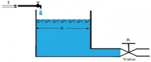
The tank structure as seen in Figure 2. Suppose μ=0 is the inflow disruption of the tank that produces friction at the liquid stage Q, ω=1 is a flow barrier that can be governed by a value.
Q=1 is the tank's cross-section. The liquid sum is assumed to be the following partnership.
$\zeta(\mathrm{t})=-\frac{1}{\mathrm{Q} \omega} \zeta(\mathrm{t})+\frac{\mu}{\mathrm{Q^{'}}} 0 \leq \mathrm{T} \leq \widetilde{\mathrm{T}}$
$\zeta(0)=(\zeta(0, \mathrm{r}), \bar{\zeta}(\mathrm{r}, 0))$
Figure 2. Liquid tank system
Using a T-transform produces the following equation:
i. $\zeta(\mathrm{t})$ be ii- differentiable, $\widetilde{\mathrm{T}}\left[\zeta^{\prime}(\mathrm{t})=-\zeta(\mathrm{t})+\frac{\mu}{\mathrm{Q}}\right]\frac{-\bar{\zeta}(0)}{\mathrm{u}}+\frac{\mathrm{T}[\overline{\bar{\zeta}}(\mathrm{t})]}{\mathrm{u}^{2}}=\mathrm{T}[-\zeta(\mathrm{t})]$
$-\mathrm{u} \bar{\zeta}(0)+\mathrm{T}[\bar{\zeta}(\mathrm{t})]=\mathrm{u}^{2} \mathrm{~T}[-\mathrm{\zeta}(\mathrm{t})]$ (5)
$-\mathrm{u} \underline{\zeta}(0)+\mathrm{T}[\zeta(\mathrm{t})]=\mathrm{u}^{2} \mathrm{~T}[-\bar{\zeta}(\mathrm{t})]$ (6)
from 5 and 6 we have:
$\mathrm{T}[\zeta(\mathrm{t})]=\frac{\mathrm{u}^{3}}{1-\mathrm{u}^{4}} \bar{\zeta}(0)+\frac{\mathrm{u}}{1-\mathrm{u}^{4}} \zeta(0)$
$\underline{\zeta}(\mathrm{t})=\sinh \mathrm{t} \bar{\zeta}(0)+\cosh \mathrm{t} \underline{\zeta}(0)$
$\bar{\zeta}(\mathrm{t})=\sinh \mathrm{t} \underline{\zeta}(0)+\cosh \mathrm{t} \bar{\zeta}(0)$
$\widetilde{\mathrm{T}}[\zeta(\mathrm{t})]=(\sinh \mathrm{t} \underline{\zeta}(0)+\cosh \mathrm{t} \bar{\zeta}(0), \sinh \mathrm{t} \underline{\zeta}(0)+\cosh \mathrm{t} \bar{\zeta}(0))$.
ii. $\zeta(\mathrm{t})$ be i- differentiable, $\widetilde{\mathrm{T}}\left[\zeta^{\prime}(\mathrm{t})\right]=\widetilde{\mathrm{T}}\left[-\zeta(\mathrm{t})+\frac{\mu}{\mathrm{Q}}\right]$
$\frac{\mathrm{T}[\underline{\zeta}(\mathrm{t})]}{\mathrm{u}^{2}}-\frac{\zeta(0)}{\mathrm{u}}=-\mathrm{T}[\zeta(\mathrm{t})]$
$\mathrm{T}[\underline{\zeta}(\mathrm{t})]-\mathrm{u}{\underline{\zeta}}(0)=-\mathrm{u}^{2} \mathrm{~T}\left[\underline{\zeta}(\mathrm{t})\right]$
$\mathrm{T}[\underline{\zeta}(\mathrm{t})]=\frac{\mathrm{u}}{1+\mathrm{u}^{2}} \underline{\zeta}(0)$
$\underline{\zeta}(t)=e^{-t} \underline{\zeta}(0)$
$\mathrm{T}[\bar{\zeta}(\mathrm{t})]=\frac{\mathrm{u}}{1+\mathrm{u}^{2}} \bar{\zeta}(0)$
$\underline{\zeta}(\mathrm{t})=\mathrm{e}^{-\mathrm{t}} \bar{\zeta}(0)$
$\widetilde{\mathrm{T}}[\zeta(\mathrm{t})]=\left(\mathrm{e}^{-\mathrm{t}}\underline{\zeta}(0), \mathrm{e}^{-\mathrm{t}} \bar{\zeta}(0)\right)$.
A modern mathematical approach is explored in this study. which is a fuzzy transformation of Tarig (T-agreement-transform) that is used for a solution of 1st order FDEs? In such a way as to explain it by extending the definition of extremely generalized differentiability. It is obvious that the FDE removes the algebraic problem from the fuzzy Tarig transformation approach. In addition, some essential theorems are given to show the properties of T-transform. In comparison, two practical results validate the new mathematical procedure. In other words, this paper provides a major contribution to the implementation of a higher starting point for such extensions. Future work would include applying this transformation to solve a system of FDEs and partial differential equations.
In our paper, we concluded that a fuzzy Tarig transformation ($\tilde{T}-$ transform) solves numerous realist problems in an easier and faster way. In more details there are two general cases, the first one, if is ii-differential odd function, the solution will be solved by compensation. Whereas the second case When cases is ii-differential odd, the solution will be by compensation. In the case of ii-differential even, the solution will be direct is ii-differential even function, the solution will be direct and depends on the upper and lower initial condition.
[1] Uzhga-Rebrov, O., Kuleshova, G. (2018). Problems of statistical processing of fuzzy initial data. In 2018 59th International Scientific Conference on Information Technology and Management Science of Riga Technical University (ITMS), pp. 1-3. https://doi.org/10.1109/ITMS.2018.8552973
[2] Lubiano, M.A., Montenegro, M., Sinova, B., de Sáa, S. D.L.R., Gil, M.Á. (2016). Hypothesis testing for means in connection with fuzzy rating scale-based data: algorithms and applications. European Journal of Operational Research, 251(3): 918-929. https://doi.org/10.1016/j.ejor.2015.11.016
[3] Michta, M. (2020). Stochastic integrals and stochastic equations in set-valued and fuzzy-valued frameworks. Stochastics and Dynamics, 20(1): 2050001. https://doi.org/10.1142/S021949372050001X
[4] Datta, D.P. (2003). The golden mean, scale free extension of real number system, fuzzy sets and 1/f spectrum in physics and biology. Chaos, Solitons & Fractals, 17(4): 781-788. https://doi.org/10.1016/S0960-0779(02)00531-3
[5] El Naschie, M.S. (2005). On a fuzzy Kähler-like manifold which is consistent with the two slit experiment. International Journal of Nonlinear Sciences and Numerical Simulation, 6(2): 95-98. https://doi.org/10.1515/IJNSNS.2005.6.2.95
[6] Kaleva, O. (1987). Fuzzy differential equations. Fuzzy Sets and Systems, 24(3): 301-317. https://doi.org/10.1016/0165-0114(87)90029-7
[7] Abbasbandy, S., Viranloo, T.A., Lopez-Pouso, O., Nieto, J.J. (2004). Numerical methods forfuzzy differential inclusions. Computers & Mathematics with Applications, 48(10-11): 1633-1641. https://doi.org/10.1016/j.camwa.2004.03.009
[8] Assmann, J., Bernstein, R., Goetschel, W., Hendel, R., Malabou, C., Schwab, G., Whitebook, J. (2018). Freud and Monotheism: Moses and the Violent Origins of Religion. Fordham Univ Press.
[9] Salahshour, S. (2011). Nth-order fuzzy differential equations under generalized differentiability. Journal of Fuzzy Set Valued Analysis, 1-14.
[10] Bede, B., Gal, S.G. (2005). Generalizations of the differentiability of fuzzy-number-valued functions with applications to fuzzy differential equations. Fuzzy Sets and Systems, 151(3): 581-599. https://doi.org/10.1016/j.fss.2004.08.001
[11] Georgiou, D.N., Nieto, J.J., Rodriguez-Lopez, R. (2005). Initial value problems for higher-order fuzzy differential equations. Nonlinear Analysis: Theory, Methods & Applications, 63(4): 587-600. https://doi.org/10.1016/j.na.2005.05.020
[12] Salahshour, S. (2011). Nth-order fuzzy differential equations under generalized differentiability. Journal of fuzzy Set Valued Analysis, 2011: 1-14.
[13] Hooshangian, L., Allahviranloo, T. (2014). A new method to find fuzzy nth order derivation and applications to fuzzy nth order arithmetic based on generalized h-derivation. An International Journal of Optimization and Control: Theories & Applications (IJOCTA), 4(2): 105-121. https://doi.org/10.11121/ijocta.01.2014.00183
[14] Goetschel Jr, R., Voxman, W. (1986). Elementary fuzzy calculus. Fuzzy Sets and Systems, 18(1): 31-43. https://doi.org/10.1016/0165-0114(86)90026-6
[15] Kaleva, O. (1987). Fuzzy differential equations. Fuzzy Sets and Systems, 24(3): 301-317. https://doi.org/10.1016/0165-0114(87)90029-7
[16] Puri, M.L., Ralescu, D.A. (1983). Differentials of fuzzy functions. J. Math. Anal. Appl., 91(2): 552-558.
[17] Dubois, D., Prade, H. (1982). Towards fuzzy differential calculus part 3: Differentiation. Fuzzy Sets and Systems, 8(3): 225-233.
[18] Chalco-Cano, Y., Roman-Flores, H. (2008). On new solutions of fuzzy differential equations. Chaos, Solitons & Fractals, 38(1): 112-119. https://doi.org/10.1016/j.chaos.2006.10.043
[19] Elzaki, T.M., Elzaki, S.M. (2011). The new integral transform Tarig Transform properties and applications to differential equations. Elixir International Journal, 38: 4239-4242.
[20] Jafari, R., Razvarz, S. (2018). Solution of fuzzy differential equations using fuzzy Sumudu transforms. Mathematical and Computational Applications, 23(1): 5. https://doi.org/10.3390/mca23010005