Jawad Kadhim Tahir
© 2021 IIETA. This article is published by IIETA and is licensed under the CC BY 4.0 license (http://creativecommons.org/licenses/by/4.0/).
OPEN ACCESS
The article studies some mathematical models that represent one class of dynamical equations in quasi-Sobolev space. The analytical investigation of solvability of the Cauchy problem in the quasi-Sobolev space and theoretical results used to enhance and develop an algorithm structure of the numerical procedures to find approximate solutions for models, the steps of algorithm based on the theoretical investigation of models, new algorithm of numerical method allowing to find approximate solutions of mathematical models under study in quasi-Sobolev space. Construction a program implements an algorithm of numerical method that allow finding approximate solutions for models. To construct the theory of degenerate holomorphic semigroups of operators in quasi-Banach spaces of sequences, we used the classical methods of functional analysis, theory of linear bounded operators, spectral theory. To construct the operators of resolving semigroups we used the Laplace transform of operator-valued functions in quasi-Banach spaces of sequences. The numerical investigation for models generate some approximate solutions which are normally based on the modified projection method. The convergence of the approximate solution to the exact one theoretically is justified by the convergence of the corresponding series, the agreement of approximate computations with the theoretical solution is established.
dynamical mathematical models, quasi-Sobolev space, projection method, Hoff model, Barenblat-Zheltov-Kochina model
Sobolev type equations as abstract operator-differential equations in terms of the relative spectrum and the results of the solvability of such equations in Banach spaces are presented by Sagadeeva and Rashid [1], Sviridyuk [2]. The concept of quasi-Banach spaces is apparently inextricably linked with the concept of Banach spaces [3, 4]. However, an independent interest in quasi-Banach spaces, as an object of research, appeared recently, moreover, such spaces arise in the study of Abelian groups [5-7] and applied problems [8, 9]. The study of dynamical equations in quasi-Banach spaces relevant due to the fact that the results obtained more than twenty years ago in Banach spaces turned out to be applicable in the theory of dynamic measurements [10-13]. Mathematical models based on linear Sobolev-type equations were studied [14-18].
The space $\ell_{q}^{r}$ is a quasi-Banach space. For all r $\in$ R. q $\in$ R_+ and $c=2^{\frac{1-q}{q}}$ .
Suppose that $P_{n}(x)=\sum_{i=0}^{n} c_{i} x^{i}$ and $Q_{m}(x)=\sum_{j=0}^{m} d_{j} x^{j}$ are polynomials with real coefficients of degrees n and m respectively such that $m \leq n$ and do not have a common root.
The class of dynamical equations in quasi-Sobolev defined by
$P_{n}(\Lambda) \dot{u}=Q_{m}(\Lambda) u$ (1)
Putting L=Pn(Λ) and M=Qm(Λ), we consider Eq. (1) in the range of the abstract equation of Sobolev type.
$L \dot{u}=M u$ (2)
where, a vector function $u \in C^{\infty}\left(\mathbb{R}_{+} ; \ell_{q}^{r+2 n}\right)$ represents a solution for (2). u=u(t) represents a solution of the Cauchy problem.
$u(0)=u_{0}$ (3)
if it satisfies (2) and the Cauchy condition (3) for some $u_{0} \in$$\ell_{q}^{r+2 n}$.
Suppose that $\mathfrak{U}$ and $\mathfrak{F}$ are quasi-Sobolev spaces, moreover L. $M \in \mathcal{L}(\mathfrak{U} ; \mathfrak{F})$. The sets of L-resolvent and L-spectrum with respect to the operator M respectively which formulated as follows:
$\begin{aligned} \rho^{L}(M)=\{\mu \in \mathbb{C}:& \left.(\mu L-M)^{-1} \in \mathcal{L}(\mathfrak{U} ; \widetilde{\mho})\right\} . \sigma^{L}(M) \\ &=\mathbb{C} \backslash \rho^{L}(M) \end{aligned}$
The relative spectral of the operator σL(M) is defined as follows:
$\sigma^{L}(M)=\sigma_{1}^{L}(M) \cup \sigma_{2}^{L}(M)$ and $\sigma_{1}^{L}(M) \neq \phi$
where there is abounded domain $\Omega_{1} \subset \mathbb{C}$ and $\partial \Omega_{1}$
of class $C^{1} . \Omega_{1} \supset \sigma_{1}^{L}(M)$ and $\Omega_{1} \cap \sigma_{2}^{L}(M)=\phi$ (4)
Now we defined the operators P1 and Q1 as follows:
$P_{1}=\frac{1}{2 \pi i} \int_{\gamma_{1}} R_{\lambda}^{L}(M) d \lambda$
and
$Q_{1}=\frac{1}{2 \pi i} \int_{\gamma_{1}} L_{\lambda}^{L}(M) d \lambda$
where,
$R_{\mu}^{L}(M)=(\mu L-M)^{-1} M, L_{\mu}^{L}(M)=M(\mu L-M)^{-1}$
are the right and left L-resolvent of an operator M and γ1 = ∂Ω1.
Definition 1. If there exists a∈R+, for each μ∈C(|μ|>a) such that μ∈ρL(M) then M a relatively spectral bounded of L and denoted by (L. σ)-bounded.
Lemma 1. If M is (L. σ)-bounded then $P_{1} \in \mathcal{L}(\mathfrak{U})$ and $Q_{1} \in \mathcal{L}(\mathfrak{F})$ are projectors.
Proof. Since the integrand operator function is analytic, then
$P_{1}=\frac{1}{2 \pi i} \int_{\gamma_{1}} R_{\lambda}^{L}(M) d \lambda$
and
$Q_{1}=\frac{1}{2 \pi i} \int_{\gamma_{1}} L_{\lambda}^{L}(M) d \lambda$
where, the contour $\dot{\gamma}_{1}$ is a bounded domain which containing the contour γ1 and not containing the points of the set $\sigma_{2}^{L}(M)$, that is it is a bit “wider” than the contour.
$P_{1}^{2}=\frac{1}{(2 \pi i)^{2}} \int_{\gamma_{1}}\int_{\gamma_{1}} R_{\lambda}^{L} R_{\mu}^{L}(M) d \mu d \lambda$
$=\frac{1}{(2 \pi i)^{2}}\left(\int_{\gamma_{1}} \frac{d \lambda}{\lambda-\mu} \int_{\gamma_{1}} R_{\mu}^{L}(M) \int_{\gamma_{1}} R_{\lambda}^{L} d \mu+\int_{\gamma_{1}} R_{\lambda}^{L}(M) d \lambda \int_{\gamma_{1}} \frac{d \mu}{\mu-\lambda}\right)$
$=\frac{1}{2 \pi i} \int_{\gamma_{1}} R_{\lambda}^{L}(M) d \lambda=P_{1}$
by virtue of Fubini’s theorem, residue theorems and relatively resolvent identities. The operator Q is proved similarly by replacement the right L-resolvent identity with the left.
Definition 2. A subspace $\mathfrak{P}$ of the quasi-Sobolev space $\mathfrak{U}$ named as a phase space for (2), if it satisfies:
i- $\forall u_{0} \in \mathfrak{B} . \exists !$ solution for (2)-(3).
ii- if u=u(t) a solution for (2) then $u \in \mathfrak{P}$ and defined as a trajectory.
Remark 1. The projectors Q1 and P1 are define the spaces $\mathfrak{U}$ and $\mathfrak{F}$ as direct sums ( $\mathfrak{U}=\mathfrak{U}^{0} \oplus \mathfrak{U}^{1}, \mathfrak{F}=\mathfrak{F}^{0} \oplus \mathfrak{F}^{1}$).
Theorem 1. [19] If M is (L. p)- bounded and $p \in\{0\} \cup \mathbb{N}$, then $\mathfrak{U}^{1}$ a phase space for (2).
Lemma 1. If $\mathfrak{U}=\ell_{q}^{r+2 n}$ and $\mathfrak{F}=\ell_{q}^{r}$ then L. $M \in \mathcal{L}(\mathfrak{U} ; \mathfrak{F})$.
Proof. By construction $L=P_{n}(\Lambda): \ell_{q}^{r+2 n} \rightarrow \ell_{q}^{r}$ linear and bounded, that is $L \in \mathcal{L}(\mathfrak{U} ; \mathfrak{F})$. An operator M=$Q_{m}(\Lambda): \ell_{q}^{r+2 n} \rightarrow \ell_{q}^{r+2(n-m)}$ for m≤n, therefore M is a linear and continuous from $\mathfrak{U}$ to $\mathfrak{F})$.
Theorem 2. [20] If λk are not common roots of the polynomials Pn(x) and Qm(x) then then the operator M is (L. p) − bounded.
Now introduce L-spectrum of operator M which possesses following form
$\sigma^{L}(M)=\left\{\mu \in \mathbb{C}: \mu_{k}=\frac{Q_{m}\left(\lambda_{k}\right)}{P_{n}\left(\lambda_{k}\right)}, P_{n}\left(\lambda_{k}\right) \neq 0\right\}$
since λk → +∞ and m≤n, the set of L-spectrum of operator M tend to a finite set of points, the set σL(M) is bounded.
Theorem 3. [1] If the operator M is (L. p)-bounded and $p \in\{0\} \cup \mathbb{N}$, then ∃! a resolution group for (2) which owns the for
$U^{t}=\frac{1}{2 \pi i} \int_{\gamma_{1}} R_{\mu}^{L}(M) e^{\mu t} d \mu, t \in \mathbb{R}_{+}$
such that $\gamma=\left\{\mu \in \mathbb{C}:|\mu|>a \cdot a \in \mathbb{R}_{+}\right\}$ which is called the contour set.
From the above theorems (2) and (3), we can define the holomorphic resolution of the Eq. (1) as follows
$U^{t}=\left\{\begin{array}{l}\sum_{k=1}^{\infty} \quad e^{\mu_{k} t}<\cdot e_{k}>e_{k} \\if P_{n}\left(\lambda_{k}\right) \neq 0\\ \sum_{k \in \mathbb{N}: k \neq \ell} e^{\mu_{k} t}<\cdot e_{k}>e_{k} . \text { if } \exists \ell \\ \in \mathbb{N} \text { such that } P_{n}\left(\lambda_{\ell}\right)=0\end{array}\right.$
A phase space of the Eq. (2) has the form:
$\mathfrak{U}^{1}=\left\{\begin{array}{l}\mathfrak{U} \text { if } P_{n}\left(\lambda_{k}\right) \neq 0 . k \in \mathbb{N} \\ \left\{u \in \mathfrak{U}: u_{\ell}=0 . P_{n}\left(\lambda_{\ell}\right)=0\right\}\end{array}\right.$
Definition 3. A subspace $\widetilde{\Im}$ of the phase space $\mathfrak{P}$ is called invariant subspace for the equation (2), if $\forall u_{0} \in \widetilde{\Im}, \exists ! u=u(t)$ as a solution for the problem (2)-(3) and $u(t) \in \Im, \forall t \in \mathbb{R}_{+}$.
Theorem 4. [2] If M is (L. p) − bounded, $p \in\{0\} \cup \mathbb{N}$ and satisfies (4), then
$U_{1}^{t}=\frac{1}{2 \pi i} \int_{\gamma_{1}} R_{\mu}^{L}(M) e^{\mu t} d \mu, t \in \mathbb{R}_{+}$
is an invariant space for the Eq. (2).
Remark 2. The solution of the Eq. (2) has exponential dichotomy if:
i- $\mathfrak{P}$ (phase space) for (2) written in the form $\mathfrak{P}=\Im{}^{1} \bigoplus \Im{}^{2}$, $\Im{}^{1}$ and $\Im{}^{2}$ are invariant spaces of the Eq. (2).
ii- for any $u_{0} \in \mathfrak{J}^{1}\left(u_{0} \in \mathfrak{J}^{2}\right), u=u(t)$ a solution for the problem (2)-(3) such that
${ }_{\mathfrak{u}}\|u(t)\| \leq C_{1} e^{-a_{1} t}{ }_{\mathfrak{u}}\left\|u_{0}\right\|\left(\mathfrak{u}\|u(t)\| \geq C_{2} e^{a_{2} t}{ }_{\mathfrak{u}}\left\|u_{0}\right\|\right)$, for some $a_{1} \cdot a_{2}>0 . t \in \mathbb{R}_{+}$.
An approximate solution of the problem (2)-(3) based on the projection method which is modified due to the fact that the problem may be degenerate.
A brief description of the essence of the numerical method to find an approximate solution $\tilde{u}(t)$ by using:
$\tilde{u}(t)=u^{N}(t)=\sum_{k=1}^{N} u_{t}(t) e_{k}$ (5)
where, $N \in \mathbb{N}$.
It is necessary when we apply the projection method to take in account firstly the effects of degeneracy of the equation, secondly fulfilment required accuracy.
To select a number N, first of all defined a required estimation by:
$\int_{0}^{T}\left(_{q}^{r}\|u(t)-\tilde{u}(t)\|\right) d t<\varepsilon$,
For given $\epsilon .$
By substituting a quasi-norm on the left side, we get:
$\int_{0}^{T}\left(\sum_{k=1}^{\infty}\left(x_{k}^{\frac{r}{2}}\left|u_{k}-\tilde{u}_{k}\right|\right)^{q}\right)^{1 / q} d t$
$=\int_{0}^{T}\left(\sum_{k=N+1}^{\infty}\left(x_{k}^{\frac{r}{2}}\left|u_{k}\right|\right)^{q}\right)^{1 / q} d t$
$=\int_{0}^{T}\left(\sum_{k=N+1}^{\infty} x_{k}^{\frac{q r}{2}} e^{q \mu_{k} t}\left|u_{k}^{0}\right|^{q}\right)^{1 / q} d t$
$\leq \int_{0}^{T}\left(_{q}^{r}\left\|u^{0}\right\| e^{\mu_{N} t}\right.$
Hence
$\mu_{N}-$$\frac{\ln \left(\varepsilon \mu_{N}+{ }_{q}^{r}\left\|u^{0}\right\|\right)-\ln \left(_{q}^{r}\left\|u^{0}\right\|\right)}{T}$$<0$ (6)
We get from (6), we find N for the approximate solution.
In addition to the degeneracy of the equation, it is necessary to take a number N large enough such that xN lies to the right of all roots of the polynomial Pn(x).
By substituting (5) in (2) for uN(x.t), we get
$\sum_{k=1}^{N} P_{n}(x) u_{k}^{\prime}(t) e_{k}=\sum_{k=1}^{N} Q_{m}(x) u_{k}(t) e_{k}$ (7)
which representing a finite system of equations, the equations in the system (8) can be differential or algebraic.
We consider the following two cases:
case 1. Pn (x)≠0. k=1.….N, in this case all the equations of the system will be first order ordinary differential equations, by solving a system, we get the unknown functional coefficients ut(t).k=1.….N, in the approximate solution $\tilde{u}(t)=$$u^{N}(x, t)$.
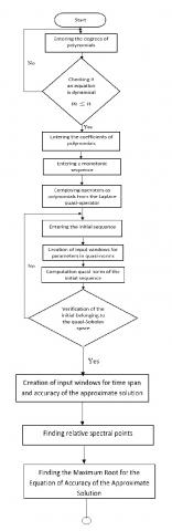
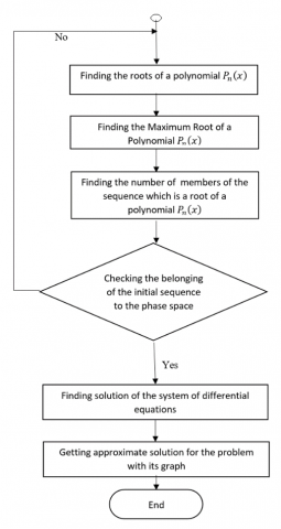
Figure 1. Diagram of approximate solution algorithm
case 2. Pn(x)=0, for some kj, in this case the equations of the system with number kj will be algebraic equations and the rest equations will be differential equations.
The steps of the algorithm finding an approximate solution for the problem (2)-(3) are:
i- finding the number N, we can find the approximate solution depend on the number N;
ii- checking mathematical model according to the given parameters to which two cases (mentioned above) it refer;
iii- calculation of the approximate solution for a given initial sequence by using a modified projection method.
The numerical study for the class dynamical mathematical models in quasi-Sobolev space based on the developed method for finding an approximate solution with a given accuracy, the numerical method was implemented by using programmable algorithm. The developed program allows us:
1- entering the polynomials which defined from the Laplace quasi-operator and consider dynamical mathematical models in quasi-Sobolev space;
2- taking into account the degeneracy of the mathematical model and apply the phase space method;
3- finding non-zero terms of an approximate solution which are necessary to fulfil a given accuracy $\epsilon .$
4- finding and deriving an approximate solution for the problem.
5- getting the graphic of the components of obtained solution depending on time.
Figure 1 shows an algorithm for finding of the approximate solution.
4.1 Computational experiments for Hoff model
Consider the analog of the linearized Hoff model
$(\lambda+\Lambda) u_{t}=\alpha u \quad \lambda \in \mathbb{R} \cdot \alpha \in \mathbb{R} \backslash\{0\}$ (8)
$u(x, 0)=u_{0} \quad x \in[0 . l]$ (9)
$u(0 . t)=u(l . t)=0 \quad t \in[0 . T]$ (10)
In quasi-Sobolev spaces $\mathfrak{U}=\ell_{q}^{r+2 n}$ and $\mathfrak{F}=\ell_{q}^{r}$ such that $r \in \mathbb{R} . q \in \mathbb{R}_{+} . L=P_{1}(\Lambda)=\lambda+\Lambda$ and $M=Q_{0}(\Lambda)=\alpha \mathbb{I}$, the operators L. $M \in \mathcal{L}(\mathfrak{U} ; \mathfrak{F})$.
Example 1. To find a numerical solution of the mathematical model (8)-(10) construct the polynomials from the Laplace quasi-operator: P1(x)=2+x and Q0=-4 where λ=2 and α=4.
Suppose that T=5. m=1. q=3. l=2π. λk=k2 and $u_{0_{k}}=\frac{1}{k^{3}}$.
Case 1. For ϵ=0.1, checking the degeneracy of the mathematical model and apply the phase space method, find the number of nonzero terms of the approximate solution $\tilde{u}(t)$ which are necessary to fulfil a given accuracy ϵ=0.1.
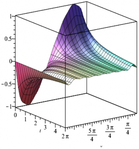
An approximate solution of the mathematical model (8)-(10) with the assuming parameters and components is
$\tilde{u}(\mathrm{x.t})=e^{-1.3333 t} \sin (x)+0.25 e^{-0.6667 t} \sin (2 x)+$$0.1111 e^{-0.3636 t} \sin (3 x)+$
$0.0625 e^{-0.2222 t} \sin (4 x)+0.04 e^{-0.1481 t} \sin (5 x)+$$0.0278 e^{-0.1053 t} \sin (6 x)+0.0204 e^{-0.0784 t} \sin (7 x)$
Figure 2 represent an approximate solution.
Figure 2. Graph for example 1 case 1
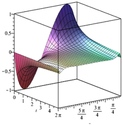
Case 2. For $\epsilon=0.01$, after getting the components of the approximate solution which necessary to fulfil a given accuracy, we get an approximate solution for (8)-(10) as follows:
$\begin{aligned} \tilde{u}(\mathrm{x} . \mathrm{t})=e^{-1.3333} t & \sin (x)+0.25 e^{-0.6667 t} \sin (2 x) \\ &+0.1111 e^{-0.3636 t} \sin (3 x) \\ &+0.0625 e^{-0.2222 t} \sin (4 x) \\ &+0.04 e^{-0.1481 t} \sin (5 x) \\ &+0.0278 e^{-0.1053 t} \sin (6 x) \\ &+0.0204 e^{-0.0784 t} \sin (7 x) \\ &+0.0156 e^{-0.0606 t} \sin (8 x) \\ &+0.0123 e^{-0.0482 t} \sin (9 x) \\ &+0.01 e^{-0.0392 t} \sin (10 x) \\ &+0.0083 e^{-0.0325 t} \sin (11 x) \\ &+0.0069 e^{-0.0274 t} \sin (12 x) \\ &+0.0059 e^{-0.0234 t} \sin (13 x) \\ &+0.0051 e^{-0.0202 t} \sin (14 x) \\ &+0.0044 e^{-0.0176 t} \sin (15 x) \\ &+0.0039 e^{-0.0155 t} \sin (16 x) \\ &+0.0035 e^{-0.0137 t} \sin (17 x) \\ &+0.0031 e^{-0.0123 t} \sin (18 x) \\ &+0.0028 e^{-0.011 t} \sin (19 x) \\ &+0.0025 e^{-0.01 t} \sin (20 x) \\ &+0.0023 e^{-0.009 t} \sin (21 x) \end{aligned}$
as shown in the Figure 3.
Figure 3. Graph for example 1 case 2
4.2 Computational experiments for Barenblat-Zheltov-Kochina Model
The Barenblat-Zheltov-Kochina model is defined by:
$(\lambda+\Lambda) u_{t}=\alpha \Lambda u \quad \lambda \in \mathbb{R} \cdot \alpha \in \mathbb{R} \backslash\{0\}$ (11)
$u(x, 0)=u_{0} \quad x \in[0 . l]$ (12)
$u(0 . t)=u(l . t)=0 \quad t \in[0 . T\rceil$ (13)
In quasi-Sobolev spaces $\mathfrak{U}=\ell_{q}^{r+2 n}$ and $\mathfrak{F}=\ell_{q}^{r}$ such that $r \in \mathbb{R} . q \in \mathbb{R}_{+} . L=P_{1}(\Lambda)=\lambda+\Lambda$ and $M=Q_{1}(\Lambda)=\alpha \Lambda$, the operators L. $M \in \mathcal{L}(\mathfrak{U} ; \mathfrak{F})$.
Example 2. To get an approximate solution of the mathematical model (11)-(13), in the beginning we define the polynomials, by using the Laplace quasi-operator and assuming of the parameters of Eq. (11) then we get:
P1 (x)=7-x and Q1=5x where λ=7 and α=5.
Assume that T=10. m=1. q=5. l=2π. λk=k3 and $u_{0_{k}}=\left\{\begin{array}{c}\frac{1}{k^{3}} \cdot k \neq 0 \\ 0 . k=0\end{array}\right.$.
Case 1. For ϵ=0.1, after checking the degeneracy of the mathematical model and apply the phase space method, we find the number of components of the approximate solution u˜(t) which are essentially to achieve a given accuracy ϵ=0.1.
An approximate solution of the mathematical model (11)-(13) with the components and assuming parameters is:
$\tilde{u}(\mathrm{x} . \mathrm{t})=e^{0.8333 t} \cos (x)+0.1111 e^{-22.5 t} \cos (3 x)+$$0.0625 e^{-8.8889 t} \cos (4 x)$, an approximate solution of the problem represented by Figure 4.
Figure 4. Graph for example 2 case 1
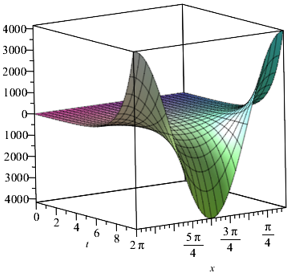
Case 2. For $\epsilon=0.01$, after computing the components of the approximate solution which necessary to fulfil a given accuracy, getting approximate solution of the mathematical model (11)-(13) with the components and assuming parameters is:
$\tilde{u}(\mathrm{x} . \mathrm{t})=e^{0.8333 t} \cos (x)+0.1111 e^{-22.5 t} \cos (3 x)$
$+\quad 0.0625 e^{-8.8889 t} \cos (4 x)$
$+0.04 e^{-6.9444 t} \cos (5 x)$
$+0.0278 e^{-6.2069 t} \cos (6 x)$
$+\quad 0.0204 e^{-5.8333 t} \cos (7 x)$
$+\quad 0.0156 e^{-5.614 t} \cos (8 x)$
$+0.0123 e^{-5.473 t} \cos (9 x)$
$++0.01 e^{-5.3763 t} \cos (10 x)$
$+\quad 0.0083 e^{-5.307 t} \cos (11 x)$
$+0.0069 e^{-5.2555 t} \cos (12 x)$
the approximate solution shown in the Figure 5.
Figure 5. Graph for example 2 case 2
1. Convergence of the numerical approach of approximate solution of mathematical models to exact one in framework of the dynamical mathematical models in quasi-Sobolev spaces theoretically is justified by the convergence of the corresponding series.
2. The numerical approach of approximate solution is appropriate, rapid and efficient to solve more complicated dynamical mathematical models, although such models take a long time when we apply other methods
3. Getting sufficient conditions for the existence of invariant spaces of solutions and their dichotomies for the class of dynamical mathematical models in quasi-Sobolev spaces.
4. Construction an algorithm for numerical method to study the class of dynamical mathematical models in quasi-Sobolev spaces.
5. Designing a program implements an algorithm of numerical method for studying of the class of dynamical mathematical models in quasi-Sobolev space.
I would like to express my thanks to the Mustansiriyah University (www.uomustansiriyah.edu.iq) in Baghdad - Iraq for encouragement and support.
|
$\mathbb{N}$ |
set of natural numbers |
|
$\mathbb{R}$ |
set of real numbers |
|
$\mathbb{R}_{+}$ |
set of positive real numbers |
|
$\mathbb{C}$ |
set of complex numbers |
|
$\mathcal{L}(\mathfrak{U})$ |
set of continuous linear operators defined on the space $(\mathfrak{U})$ |
|
$\ell_{q}$ |
space of sequences |
|
$u_{t}$ |
partial derivative of $u$ with respect to t |
|
$C^{\infty}$ |
space of the infinitely differentiable functions |
|
$r \\q$$\|\cdot\|$ |
quasi-norm |
[1] Sagadeeva, M.A., Rashid, A.S. (2015). Existence of solutions in quasi-Banach spaces for evolutionary Sobolev type equations in relatively radial case. Journal of Computational and Engineering Mathematics, 2(2): 71-81. https://doi.org/10.14529/jcem150207
[2] Sviridyuk, G.A. (1994). On the general theory of operator semigroups. Russian Mathematical Surveys, 49(4): 45-74. https://doi.org/10.1070/RM1994v049n04ABEH002390
[3] Bastero, J., Bernues, J., Pena A. (1995). An extention of Milmans Reverse Burn–Minkowski inequality. Mathematics, 1: 950-1210.
[4] Berg, I., Lofstorm, I. (1980). Interpolation spaces. MIR Publishers Moscow (in Russian).
[5] Hardtke, J.D. (2013). A remark on condensation of singularities. Journal of mathematical physics, analysis, Geometry, 9(4): 448-454.
[6] Kalton, N. (2003). Quasi-Banach Spaces, Handbook of the Geometry of Banach Spaces. Johnson, WB, Lindenstrauss, J., Elsevier, (eds.), 2: 1099-1130. https://b-ok.org/book/504198/e055e6
[7] Keller, A., Zamyshlyaeva, A., Sagadeeva, M. (2015). On integration in quasi-banach spaces of sequences. Journal of Computational and Engineering Mathematics, 2(1): 52-56. https://doi.org/10.14529/jcem150106
[8] Kim, J.S. (2005). A continuous surface tension force formulation for diffuse interface models. Journal of computational Physics, 204(2): 784-804. http://www.math.uci.edu/~jskim.
[9] Novikov, S.Y. (1997). Singularities of embedding operators between symmetric function spaces on [0, 1]. Mathematical Notes, 62(4): 457-468. https://doi.org/10.1007%2FBF02358979
[10] Chshiev, A.G. (2011). Spectral analysis of degenerate semigroups Operators. Dissertation Candidate Phys.-Math. Science, Voronezh. (in Russian).
[11] Favini, A., Yagi, A. (1998). Degenerate Differential Equations in Banach spaces. CRC Press.
[12] Fedorov, V.E. (2008). Holomorphic operator semigroups with strong degeneration. Bulletin of Chelyabinsk State University, 10: 68–74 (in Russian). http://www.mathnet.ru/php/archive.phtml?wshow=paper&jrnid=vchgu&paperid=96&option_lang=eng.
[13] Kakushkin, S.N., Kadchenko, S.I. (2016). The calculation of values of eigenfunctions of the perturbed self-adjoint operators by regularized traces method. Journal of Computational and Engineering Mathematics, 2(4): 48-60. https://doi.org/10.14529/jcem150405
[14] Sviridyuk, G.A. (1987). Cauchy problems for a linear singular equation of Sobolev type. Differential Equations, 23(12): 2169-2171.
[15] Sviridyuk, G.A. (1994). Phase portraits of Sobolev-type semilinear equations with a relatively strongly sectorial operator. Algebra and Analiz, 6(5): 252-272.
[16] Sviridyuk, G.A., Fedorov, V.E. (2003). Linear Sobolev Type Equations and Degenerate Semigroups of Operators. Utrecht, Boston, Koln: VSP.
[17] Sviridyuk, G.A., Manakova, N.A. (2014). The dynamical models of Sobolev type with Showalter–Sidorov condition and additive “Noise”. Vestnik Yuzhno-Ural'skogo Universiteta. Seriya Matematicheskoe Modelirovanie i Programmirovanie, 7(1): 90-103. https://doi.org/10.14529/mmp140108
[18] Zamyshlyaeva, A.A. (2011). The Phase Space of Sobolev Type Equations of High Order. Izvestiya Irkutskogo gosudarstvennogo universiteta. Seriya" Matematika"[The Bulletin of Irkutsk State University. Series" Mathematics"], 4(4): 45.
[19] Sviridyuk, G.A., Kazak, V.O. (2002). The phase space of an initial-boundary value problem for the Hoff equation. Mathematical Notes, 71(1-2): 262-266. https://doi.org/10.1023/A:1013919500605
[20] Sagadeeva, M.A., Hasan, F.L. (2015). Existence of invariant spaces and exponential dichotomies of solutions for dynamical Sobolev type equations in quasi-Banach spaces. Bulletin of the South Ural State University. Series: Mathematics. Mechanics. Physics, 7(4): 50-57. https://doi.org/10.14529/mmph150406