Arief Goeritno
© 2021 IIETA. This article is published by IIETA and is licensed under the CC BY 4.0 license (http://creativecommons.org/licenses/by/4.0/).
OPEN ACCESS
This paper describes a theoretical approach by making ordinary differential equations for observing the phenomena of temperature changes as a form of heat transfer on a single rectangular plate fin. Based on what has been done, these research objectives are obtained the phenomena of temperature change (a) as a function of the length in the copper bar and (b) as a function of the time in a fluid. The methods used in this simulation are: (i) do the simplification of differential equations with several assumptions to obtain the final form of differential equations and (ii) do a simulation based-on spreadsheet application to obtain a curve of temperature change. The simulation results are in the form of a change curve, i.e. (a) the temperature change in the copper bar as a function of length and (b) changes in temperature values on the fluid as a function of time. In general, it is concluded, that changes in the value of parameters as a function of the distance or the time can be done by making the ordinary differential equations models, so that can be implemented in the simulation process.
observing the phenomena of temperature changes, ordinary differential equations models, single rectangular plate fin
Models describe the beliefs about how the world functions. In mathematical modeling, those beliefs must be translated into the language of mathematics. There is a lot of element of compromise in the mathematical modeling that can be used for several different reasons [1, 2]. To apply some mathematical methods to a "real-life" problem or is called physical problems, must be formulated the problem in mathematical terms, i.e. must be constructed a mathematical model for the problem [3]. Many physical problems concern relationships between changing quantities, namely since rates of change are represented mathematically by derivatives. The mathematical models often involve equations relating to an unknown function and one or more of its derivatives. Such equations are differential equations [3].
Geometric equations and physical problems have become evident as information givers [4] for some of the features of the differential equations [4-8]. Some important problems in engineering, physics, and social sciences, when informed in mathematical form, require research of a function by fulfilling a problem containing one or more derivatives of an unknown function [8]. Manifestation is the form of language in the formulation and resolution of problems in science and engineering is one of the important roles of ordinary differential equations [9, 10]. The existence of ordinary differential equations is characterized by a clear classification of dependence on only one variable. One such variable can be time, distance, or the other [4-10].
The implementation of various fin geometries (rectangular, circular, square, and elliptic) has similarities in terms of wetting surface area in terms of the point of view of heat transfer, tensile strength, and the rate of generation of total dimensionless entropy [11]. Cooling states in the fin geometry are a form of implementation of Newton's Law that the rate of change of the temperature of an object is proportional to the difference between its temperature and the temperature of its surroundings [11]. The heat that is removed from the process in the fin geometry known as a cooling process which is a physical operation [12]. The use of material for making fin is a very important factor because it is related to the heat conductivity of the material. The existence of copper material was chosen, because it is closely related to high conductivity, besides that copper material is much cheaper when compared to other materials which have the same conductivity [13, 14].
In the phenomena of heat transfer, there is a temperature difference, because the transfer of heat will continue as long as there is a difference in temperature between the two locations. In any situation results from energy flow into a system is leads to heating or energy flow from a system to surroundings is leads to cooling [15, 16]. Newton's Law makes a statement about an instantaneous rate of change of the temperature. Newton's Law makes a statement about an instantaneous rate of change of the temperature [14], then this verbal statement translated into an equation of differential. The solution to this equation is a function that tracks the complete record of the temperature, time over time. Newton's Law was enabled to solve that problem [17].
Implementing a single rectangular plate fin as a passive heat exchanger for a fluid cooling process is an application of differentiation to solve the temperature parameter value per unit of distance or time. Based on several descriptions, these objectives of the simulation are obtained the phenomena of temperature change, namely (i) as a function of the length in the copper bar and (ii) as a function of the time in a fluid.
2.1 Materials
2.1.1 ODEs that implemented on methods of analytical
The mathematical approach based on analytical and numerical methods for solutions on the temperature difference phenomenon with example the cooling process is carried out through the implementation of ordinary differential equations with variables x, y, and derivatives of y to x, is shown in Eq. (1) [4-10].
$F\left(x, y, \frac{d}{d x} y, \frac{d^{2}}{d x^{2}} y, \cdots, \frac{d^{n}}{d x^{n}} y\right)=0$ (1)
The form of linear equations with order-n can be written as Eq. (2).
$a_{0}(x) \frac{d^{n}}{d x^{n}} y+a_{1}(x) \frac{d^{n-1}}{d x^{n-1}} y+\cdots+a_{n-1}(x) \frac{d}{d x} y$$+a_{n}(x) y=f(x)$ (2)
where, $a_{0}, a_{1}, \cdots, a_{n-1}, a_{n},$ and $f$ is a free variable function $x$ and $a_{0} \neq 0$.
Ordinary differential equations such as Eq. (2) can be solved by methods of analytical (exact) and/or numerical (approximation) [18-21].
Analytic solution to the cooling process based on the Eq. (2), if:
#i) n=1, called linear differential equations of order-1, as shown in the Eq. (3), i,e.
$\frac{d}{d x} y+P(x) y=Q(x)$ (3)
#ii) $Q(x)=0,$ hence $\frac{d}{d x} y+P(x) y$ the order of homogeneous linear differential equations of order-1, with a general solution is shown in the Eq. (4), i.e.
$y=K \cdot e^{-\int P(x) d x}$ (4)
#iii) $Q(x) \neq 0,$ hence $\frac{d}{d x} y+P(x) y=Q(x)$ is called a non-homogeneous differential equation with a general solution is shown in Eq. (5), i.e.
$y=K \cdot e^{-\int P(x) d x}+e^{-\int P(x) d x} \cdot \int e^{-\int P(x) d x} \cdot Q(x)$$\cdot d x$ (5)
where, K is an integration constant according to boundary conditions.
2.1.2 Equation of energy balance in a single rectangular plate fin
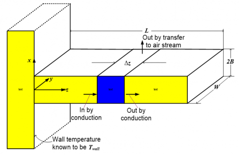
Another simple, but practical, application of heat conduction is in the calculation of the efficiency of a cooling fin. Such fins are used to increase the area available for heat transfer between metal walls and poorly conducting fluids such as gases [22]. A single rectangular plate fin with a thickness much smaller than lengthiness (B << L) is shown in Figure 1.
Figure 1. A single rectangular plate fin with a thickness much smaller than lengthiness (B << L)
A reasonably good description of the system may be obtained by approximating the true physical situation by a simplified model [22]. The comparison between the true situation and model [22] is shown in Table 1.
Table 1. The comparison between true situation and model
|
True Situation |
No. |
Model |
|
T is a function of both axis (x and z), but the dependent on the z-axis more important |
1 |
T is a function of the z-axis alone |
|
A small quantity of heat is lost from the fin at the end (area 2BW and the edges (area 2BL+2BL) |
2 |
No heat is lost from the end or the edges |
|
The heat transfer coefficient is a function of position |
3 |
The heat flux at the surface is given by q=h(T-Ta), in which h is constant and T=T(z) |
A thermal energy balance on a segment Δz of the bar gives the Eq. (6) [22].
$\left.q_{z}\right|_{z} \cdot 2 B W-\left.q_{z}\right|_{z+\Delta z} \cdot 2 B W-h(2 W \cdot \Delta z)\left(T-T_{a}\right)=0$ (6)
Division by 2BW$\cdot$Δz and taking the limit Δz approaches zero gives as the Eq. (7).
$-\frac{d}{d z} q_{z}=\frac{h_{m e t}}{B}\left(T-T_{a}\right)$ (7)
Insertion of [22] Fourier's Law $\left(q_{z}=-k \frac{d}{d z} T\right)$ in which k thermal conductivity of the metal gives for constant kmet, so that the Eq. (7) transformed into the Eq. (8).
$-\frac{d^{2}}{d z^{2}} T=\frac{h_{m e t}}{k_{m e t} \cdot B}\left(T-T_{a}\right)$ (8)
Implementation of the fin form in fluid, then the Eq. (8) changes to the Eq. (9) [22].
$-\frac{d^{2}}{d z^{2}} T=\frac{h_{m e t}}{k_{m e t} \cdot B}\left(T-T_{f}\right)$ (9)
In the case of using copper material for the simulation process, then $T=T_{c u}, h_{m e t .}=h_{c u},$ and $k_{m e t .}=k_{c u}$, so the Eq. (9) transformed into the Eq. (10).
$-\frac{d^{2}}{d z^{2}} T_{c u}=\frac{h_{m e t .}}{k_{m e t} \cdot B}\left(T_{c u}-T_{f}\right)$ (10)
The Eq. (10) is to be solved with the BC [22], at z=0, then $T_{c u}=T_{w}$ as the $1^{\text {st }} \mathrm{BC}$ and at $z=L,$ then $\frac{d}{d z} T_{c u}=0$ as the 2nd BC.
Now introduce the following dimensionless quantities [22] are shown as Eqns. (11), (12), and (13).
$\Theta=\frac{T_{c u}-T_{f}}{T_{w}-T_{f}}=$ dimensionless temperature (11)
$\zeta=\frac{z}{L}=$ dimensionless distance (12)
$N=\sqrt{\frac{h_{c u} \cdot L^{2}}{k_{c u} \cdot B}}=$ dimensionless heat transfer coefficient (13)
This problem may be restated to Eq. (14).
$\frac{d^{2}}{d \zeta^{2}} \Theta=N^{2} \Theta$ (14)
where: $\left.\Theta\right|_{\zeta=0}=1$ and $\left.\frac{d}{d \zeta} \Theta\right|_{\zeta=1}=0$.
Eq. (14) may be integrated to give hyperbolic functions [22]. When the two integration constants have been determined, so Eq. (15) is obtained [22].
$\Theta=\cosh N \zeta-(\tanh N) \cdot \sinh N \zeta$ (15)
2.2 Methods
Several equations are known, then a spreadsheet-based simulation process is carried out. The results obtained are (i) a change in temperature in the copper bar is affected by the length of the copper bar and (ii) changes in the value of the working fluid temperature. The two changes obtained are an increase in temperature as a function of the length of the copper bar and a decrease in temperature curve as a function of time. A simulation for a change in temperature in the copper bar as a function of the length of the copper bar. Further elaboration of the equation is carried out to obtain the form of a new equation that is used for simulating the temperature changes as a function of time in the vessel chamber.
3.1 Temperature change as a function of the length of a copper bar
For the acquisition of the benefit of Eq. (15), it is necessary to stage the simplification, to obtain the form of the equation that has been explained by Bird et al. [22]. The simplification process for the Eq. (18) is carried out through stages, i.e.:
#the 1st stage: $\Theta=\cosh N \zeta-\left(\frac{\sinh N}{\cosh N}\right) \cdot \sinh N \zeta$
#the 2nd stage: $\Theta=\frac{\cosh N}{\cosh N} \cdot \cosh N \zeta-\left(\frac{\sinh N}{\cosh N}\right) \cdot \sinh N \zeta$
#the 3rd stage: $\Theta=\frac{\cosh N \cdot \cosh N \zeta-\sinh N \cdot \sinh N \zeta}{\cosh N}$
After staging, it is as explained by Bird et al. [2], so that the final equation is obtained as the Eq. (16).
$\Theta=\frac{\cosh N(1-\zeta)}{\cosh N}$ (16)
The dimensionless numbers in Eqns. (11), (12), and (13) are substituted into the Eq. (16), so the Eq. (17) is obtained.
$\frac{T_{c u}-T_{f}}{T_{w}-T_{f}}=\frac{\cosh \left[\sqrt{\frac{h_{c u} \cdot L^{2}}{k_{c u} \cdot B}} \cdot\left(1-\frac{Z}{L}\right)\right]}{\cosh \sqrt{\frac{h_{c u} \cdot L^{2}}{k_{c u} \cdot B}}}$ (17)
The simplification of Eq. (17) is obtained the Eq. (18).
$T_{c u}-T_{f}=\frac{\cosh \left[\sqrt{\frac{h_{c u} \cdot L^{2}}{k_{c u} \cdot B}} \cdot\left(1-\frac{Z}{L}\right)\right]}{\cosh \sqrt{\frac{h_{c u} \cdot L^{2}}{k_{c u} \cdot B}}} \cdot\left(T_{w}-T_{f}\right)$ (18)
Further simplification to the Eq. (18), obtained the Eq. (19).
$T_{c u}=\frac{\cosh \left[\sqrt{\frac{h_{c u} \cdot L^{2}}{k_{c u} \cdot B}} \cdot\left(1-\frac{Z}{L}\right)\right]}{\cosh \sqrt{\frac{h_{c u} \cdot L^{2}}{k_{c u} \cdot B}}} \cdot\left(T_{w}-T_{f}\right)+T_{f}$ (19)
The simulation process assisted by the spreadsheet application in Eq. (19) results in a temperature change curve on the copper bar. The change in temperature value in the copper bar as a function of the length is shown in Figure 2.
Figure 2. The change in temperature value in the copper bar as a function of the length
Based on Eq. (19) and Figure 2 can be explained, that change in temperature value (in a copper bar) as a function of the length (as the distance) is shaped exponential curve with an initial length value of zero meters. It is shown that the change in temperature in the copper bar is influenced by the length of the copper bar in the form of a single rectangular plate fin.
3.2 Temperature change as a function of the time in a fluid
The rate of change of energy in a system in the form of a chamber filled with water with a cooling source from a fin rod is a simple block made of copper, equal to the rate of energy entry minus the rate of energy coming out plus the formation of energy. Referring to the statement referred to, then obtained the Eq. (20).
$\begin{aligned} m_{f} \cdot C_{p_{f}} \cdot & \frac{d}{d t} T_{f}=-h_{c u} \cdot A_{c u} \cdot\left(T_{c u}-T_{f}\right) \\ &+U_{w} \cdot A_{w} \cdot\left(T_{f}-T_{w}\right) \end{aligned}$ (20)
A solution to Eq. (20) to determine the change in fluid temperature with a change in time is obtained the Eq. (21).
$\frac{d}{d t} T_{f}=-\frac{h_{c u} \cdot A_{c u}}{m_{f} \cdot C_{p_{f}}} \cdot\left(T_{c u}-T_{f}\right)+\frac{U_{w} \cdot A_{w}}{m_{f} \cdot C_{p_{f}}}$$\cdot\left(T_{f}-T_{w}\right)$ (21)
For observations of changes in temperature values in fluids, it is necessary to value properties related to materials and fluids, namely heat capacity of copper, area of copper, a mass of fluid, heat capacity of fluid, over-all heat transfer coefficient of a wall, and area of the wall. Assumed the IC, namely (i) value of time is t= 0, (ii) temperature of copper is Tcu = 0℃, and fluid temperature is Tf= 20℃. The BC is also assumed to be a value of time is t≥0, including the temperature of the wall and the temperature of ambient air, which are considered constant. Using Eq. (21) for obtaining a change in the value of the working fluid temperature concerning time, and the curve in the form of a cooling time statement, i.e. the curve of the relationship of the temperature value to the change in time.
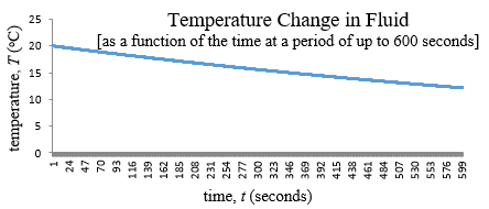
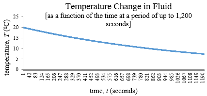
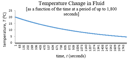
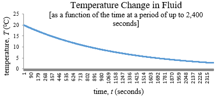
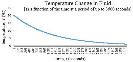
Changes in temperature values (in fluid) as a function of the time at the six various range of time is shown in Figure 3.
Figure 3. Changes in temperature values (in fluid) as a function of the time at the six various range of time
Based on Figure 3 can be explained, that change in temperature value (in fluid) as a function of the time at six various range of time with an initial temperature value of 20 degrees. The observation with a period of up to 600 seconds indicated, that the curve is formed as a straight line or linear curve.
When the observation with a period of up to 1,200 seconds, the shape of the curve changes not purely a straight line anymore. So it is the time of observation with a period of up to 1,800 seconds and up to 2,400 seconds, the shape of the curve changes to be a semi-straight line, while the time of observation with the time of up to 3,000 seconds and up to 3,6000 seconds indicated, that the curve that occurs is an exponential line curve or nonlinear curve. As a whole, it can be concluded, that the phenomena of decreasing temperature are in the form of an exponential line curve when carried out over a relatively long time.
Based on results and discussions can be concluded according to the first research objectives, that change in temperature value (in a copper bar) as a function of the length (as the distance) is shaped exponential curve with an initial length value of zero meters. It is shown that the change in temperature in the copper bar is influenced by the length of the copper bar in the form of a single rectangular plate fin. According to the second research objectives, that change in temperature value (in fluid) as a function of the time with an initial temperature value of 20 degrees is shaped linear curve when at the beginning of the time with a time of up to 600 seconds (10 minutes), then it turns into an exponential line curve. It is shown that the temperature change in the fluid is influenced by time. In general, it is concluded, that changes in the value of parameters as a function of the distance or the time through the simulation can be done by making mathematical equations based on ordinary differential equations.
Submitting of thanks to Prof. Dr. Kamaruddin Abdullah who had given the science and knowledge of the transport phenomena subjects in the lecturing on several years ago.
|
x |
dependent variable; x-axis |
|
y |
independent variable; y-axis |
|
F, P, Q, f |
functions |
|
K |
an integration constant according to boundary conditions |
|
d |
differentiating |
|
e |
exponential number = 2.71828… |
|
∫ |
integrating |
|
∑ |
summing |
|
Δ |
the segment of a |
|
n |
constant |
|
! |
factorial |
|
B |
fin thickness |
|
L |
fin lengthiness |
|
W |
fin widths |
|
z |
z-axis |
|
q |
heat flux at the surface |
|
h |
heat transfer coefficient |
|
T |
absolute temperature |
|
k |
thermal conductivity, W.m-1. K-1 |
|
Cp |
specific heat, J. kg-1. K-1 |
|
t |
time |
|
U |
over-all heat transfer coefficient |
|
A |
area, m2 |
|
BC |
boundary conditions |
|
IC |
initial conditions |
|
Greek symbols |
|
|
$\Theta$ |
dimensionless temperature |
|
$\zeta$ |
dimensionless distance |
|
N |
dimensionless heat transfer coefficient |
|
Superscripts |
|
|
1, 2, n, n-1 |
sequence to |
|
(n) |
n-th derivative |
|
Subscripts |
|
|
1, w, n |
sequence to |
|
met. |
metal |
|
cu |
copper |
|
a |
air |
|
f |
fluid |
|
w |
wall |
|
z |
in Z-axis |
[1] Lawson, D., Marion, G. (2008). An Introduction to Mathematical Modelling. Bioinformatics and Statistics Scotland, Edinburgh.
[2] Bender, E.A. (1978). An Introduction to Mathematical Modeling. John Wiley & Sons, Inc., New Jersey, 1-5.
[3] Trench, W.F. (2001). Elementary Differential Equation. Books/Cole Thomson Learning, Pacific Grove, 2.
[4] Hestenes, D. (2011). The Shape of Differential Geometry in Geometric Calculus). In: Dorst, L., Lasenby, J. (eds.) Guide to Geometric Algebra in Practice. Springer Verlag, Heidelberg, 393-410.
[5] Tenembaum, M., Pollard, H. (1985). Ordinary Differential Equations: An Elementary Textbook for Students of Mathematics, Engineering, and the Sciences. Dover Publications, Inc., New York.
[6] Coddington, E.A., Levinson, N. (1987). Theory of Ordinary Differential Equations (9-th Reprinted). Tata McGraw-Hill Publishing Co Ltd, New Delhi.
[7] Archibald, T., Fraser, C., Grattan-Guinness, I. (2004). The History of Differential Equations. Mathematisches Forschungsinstitut Oberwolfach Report. https://www.doi.org/10.4171/OWR/2004/51
[8] Logan, J.D. (2011). A First Course in Differential Equations, Second Edition. Springer Science+Business Media, New York.
[9] Dios, A.Q., Encinas, A.H., Vaquero, J.M., del Rey, A.M., Pérez, J.J.B., Sánchez, G.R. (2015). How Engineers deal with Mathematics solving Differential Equation. Procedia Computer Science, 15: 1977-1982. https://www.doi.org/10.1016/j.procs.2015.05.462
[10] Ming, C.Y. (2017). Solution of differential equations with applications to engineering problems. Dynamical Systems-Analytical and Computational Techniques. InTechOpen Limited, London. http://dx.doi.org/10.5772/67539
[11] Khan, W.A., Culham, J.R., Yovanovich, M.M. (2006). The role of fin geometry in heat sink performance. Journal of Electronic Packaging, Transactions of the ASME, 128: 324-330. http://www.doi.org/10.1115/1.2351896
[12] Joel, A.S., El-Nafaty, U.A., Makarfi, Y.I., Mohammed, J., Musa, N.M. (2017). Study of the effect of fin geometry on cooling process of computer microchips through modelling and simulation. International Journal of Industrial and Manufacturing Systems Engineering, 2(5): 48-56. https://www.doi.org/10.11648/j.ijimse.20170205.11
[13] Ashby, M., Cope, E., Cebon, D. (2013). Materials Selection for Engineering Design. In: Rajan, K. (ed) Informatics for Materials Science and Engineering: Data-driven Discovery for Accelerated Experimentation and Application, 1st Edition (reprint). Elsevier - Health Sciences Division, Woburn, USA, 219-244.
[14] Lavakumar, A. (2017). Concepts in Physical Metallurgy: Concise lecture notes. Morgan & Claypool Publishers, San Rafael, California, USA. https://www.doi.org/10.1088/978-1-6817-4473-5
[15] Adams, J.A., Rogers, D.F. (1973). Computer Aided Heat Transfer Analysis. McGraw-Hill, New York.
[16] Lienhard, I.V.J.H., Lienhard. V.J.H. (2019). A Heat Transfer Textbook, 5th ed. Phlogiston Press, Cambridge, Massachusetts, USA. https://ahtt.mit.edu/wp-content/uploads/2019/08/AHTTv500.pdf
[17] Besson, U. (2012). The history of the cooling law: When the search for simplicity can be an obstacle. Science & Education, 21: 1085-1110. https://doi.org/10.1007/s11191-010-9324-1
[18] Atkinson, K.E., Han, W., Stewart, D.E. (2009). Numerical Solution of Ordinary Differential Equations. John Wiley & Sons, Inc., Hoboken, NJ, p. 43. http://dx.doi.org/10.1002/9781118164495
[19] Farago, I., Georgiev, K., Havasi, A., Zlatev, Z. (2013). Efficient numerical methods for scientific applications: Introduction. Computers & Mathematics with Applications. 65(3): 297-300. http://dx.doi.org/10.1016/j.camwa.2013.01.001.
[20] Suli, E. (2014). Numerical Solution of Ordinary Differential Equations, Flooved.com, London, 1. http://www.flooved.com/reader/1085.
[21] Zlatev, Z., Istvan Farago, I., Havasi, A. (2014). Mathematical Treatment of Environmental Models. In: Fontes, M., Gunther, M., Marheineke, N. (eds) Progress in Industrial Mathematics at ECMI 2012, Mathematics in Industry 19, Springer International Publishing, Switzerland, 65-70. http://dx.doi.org/10.1007/978-3-319-05365-3_10
[22] Bird, R.B., Stewart, W.E., Lightfoot, E.N. (1960). Transport Phenomena. John Wiley, Singapore.