Shina D. Oloniiju* | Sicelo P. Goqo | Precious Sibanda
© 2020 IIETA. This article is published by IIETA and is licensed under the CC BY 4.0 license (http://creativecommons.org/licenses/by/4.0/).
OPEN ACCESS
We focused on developing an accurate numerical scheme for the flow of a fractional-order Oldroyd–B fluid model with the non-isothermal property. In many cases, the direct application of the Chebyshev tau method using the operational matrix of the Chebyshev polynomials usually leads to an accurate solution. However, in some cases, dealing with non–linearity and coupling can be tedious. In this study, we present a numerical method based on Chebyshev polynomials of the first kind and interpolation using Gauss–Lobatto quadrature. The coefficients of the series expansion of the pseudospectral method are obtained through integration of the Chebyshev polynomials orthogonality condition. The numerical results show that the scheme is accurate and reliable. The effects of the fractional-order objective stress rate of the Oldroyd–B fluid on the velocity and shear stress are also presented. The error bound theorems presented in this study support the findings of the numerical computations.
MHD fluid, non-isothermal flow, fractional calculus, Chebyshev – Gauss – Lobatto quadrature, fractional Oldroyd–B fluid
The Oldroyd–B fluid is a rate type model for viscoelastic fluids that have been studied extensively since its formulation by Oldroyd [1]. This model is part of a large class of rate type viscoelastic fluids models, which include, but are not limited to the upper convected Maxwell model, Jeffrey model and Burgers’ model. The Oldroyd-B model gives a good representation of the rheological response of viscoelastic fluids in shear flow. The Cauchy stress tensor for the classical Oldroyd–B constitutive model has the form
$S_{i j}=-p \delta_{i j}+\tau_{i j}$ (1)
$[1+\lambda \overset{\nabla }D] \tau_{i j}=\mu\left[1+\lambda_{r} \overset{\nabla }{D}\right]e_{ij}$ (2)
where, τij is the extra stress tensor, eij is the stress tensor. The material parameters μ, λ and λr are the viscosity, stress relaxation time and retardation time respectively and $\overset{\nabla }{D}$ is the upper convected time derivative. The constitutive model of the Oldroyd–B is a generalization of the Maxwell fluid model [2]. Unlike the Maxwell model, the Oldroyd–B fluid uses the objective stress rate that takes into account frame indifference of the deformation rate. The deformation rate is represented by the upper convected derivative in Eq. (2). Because of the memory retention characteristics of viscoelastic fluids, recent studies have suggested using non–local time derivatives [3]. Non–local objective stress rate exhibits complex dynamical and viscoelastic behaviours. Taking advantage of the inherent non–locality and memory retention characteristics of fractional derivatives, we generalize the Oldroyd–B constitutive relation by replacing the local time derivatives in Eq. (2) with fractional time derivative [4]:
$\left[1+\lambda^{\alpha}\overset{\nabla }{{\mathrm{D}}^{\alpha}}\right] \tau_{i j}=\mu\left[1+\lambda_{r}^{\beta}\overset{\nabla }{{\mathrm{D}}^{\beta}}\right] e_{i j}$ (3)
where,
$\overset{\nabla }{D^{\alpha}}=\frac{\partial^{\alpha} \tau}{\partial t^{\alpha}}+\mathbf{U} \cdot \nabla \tau-\tau \nabla \mathbf{U}-(\nabla \mathbf{U})^{\mathrm{T}} \tau$ (4)
In the constitutive model Eq. (3), 0<α, β≤1 and μ, λ, λr>0. If α>β, it should be noted that the model is physically unrealistic. This case corresponds to an increasing relaxation function [5]. Hence, the constraint on the order of the derivatives must satisfy 0<α≤β≤1. It is evident that if α=β=1, the constitutive relation is the classical Oldroyd–B fluid. Setting λr to zero in Eq. (3) corresponds to the fractional Maxwell fluid, if λ=0, the model is equivalent to the fractional second-grade fluid, if 0<λr<λ, we obtain the fractional Jeffrey fluid [6] and when λ=λr=0, the model corresponds to the classical Newtonian fluid. If we consider an incompressible fluid with constant pressure and using established notation, the momentum conservation equation for an unsteady flow of a magnetohydrodynamic (MHD) fluid is:
$\rho\left[\frac{\partial \mathbf{U}}{\partial t}+\mathbf{U} \cdot \nabla \mathbf{U}\right]=\nabla \tau_{i j}-\sigma B_{0}^{2} \mathbf{U}$ (5)
where, ρ is the fluid density, σ is the electrical conductivity of the fluid and B0 is the applied magnetic field. To write the conservation equation and the shear stress relation in non–dimensional form, we assume a reference length L and velocity $\mathbf{U}_{0},$ so that we define $t=\tilde{t} \mathbf{L} \mathbf{U}_{0}^{-1}, \mathbf{y}=\tilde{\mathbf{y}} \mathbf{L}$ for all $\mathbf{y}$ in the domain of the flow, $\mathbf{U}(\mathbf{y}, t)=\mathbf{U}_{0} \widetilde{\mathbf{U}}(\tilde{\mathbf{y}}, \tilde{t}), \tau_{i j}(\mathbf{y}, t)=$$\mathbf{U}_{0} \mu \mathbf{L}^{-1} \tilde{\tau}_{i j}(\tilde{\mathbf{y}}, \tilde{t}),$ and $\lambda_{r}=\tilde{\lambda}_{r} \mathbf{L} \mathbf{U}_{0}^{-1} .$ Therefore, we write Eq. (3) and Eq. (5) in the dimensionless form (dropping the tilde for convenience):
$\operatorname{Re}\left[\frac{\partial \mathbf{U}}{\partial t}+\mathbf{U} \cdot \nabla \mathbf{U}\right]=\nabla \tau_{i j}-H a^{2} \mathbf{U}$ (6)
$\left[1+W e^{\alpha}\overset{\nabla }{{D}^{\alpha}}\right] \tau_{i j}=\left[1+\lambda_{r}^{\beta}\overset{\nabla }{{\mathrm{D}}^{\beta}}\right] e_{i j}$ (7)
Here, $R e=\rho \mathbf{L U}_{0} \mu^{-1}$ is the Reynolds number, $H a=$ $B_{0} \mathbf{L}(\sigma / \mu)^{1 / 2}$ is the Hartmann number, $W e=\mathbf{U}_{0} \lambda \mathbf{L}^{-1}$ is the Weissenberg number, λr is a dimensionless retardation parameter. Some special cases of interest include the Jeffrey fluid (0<λr<We), Maxwell fluid (λr=0), second-order fluid (We=0), Newtonian fluid (We=λr=0) and hydrodynamic fluids (Ha=0).
Exact solutions to fractional partial differential equations are, in general, challenging to find. Even when found, the solution may contain complicated integrals and special functions that have to be approximated numerically. Several studies have proposed various methods, both numerical and analytic, for solving fractional differential equations [7-12]. However, recent studies have identified spectral methods as efficient for approximating solutions of fractional partial differential equations. Spectral methods are favoured because of their spectral rate of convergence and accuracy, especially for differential equations with sufficiently smooth solutions. Doha et al. [13] and Atabakzadeh et al. [14] presented the operational matrix of the shifted Chebyshev polynomial and used the polynomial to approximate multi-order fractional ordinary differential equations. Liu et al. [15] presented numerical solutions to multiterm variable-order fractional ordinary differential equations using the Chebyshev polynomial of the second kind as the basis function. Operational matrices of the shifted Chebyshev wavelets, generalized Laguerre polynomials, and Bernstein polynomials are presented in the studies of Benattia and Belghaba [16], Bhrawy and Alghamdi [17], Baseri et al. [18] respectively. These matrices are used to approximate the solutions of fractional differential equations. The numerical results that were reported in the studies as mentioned earlier are typical of spectral method, and they exhibit the spectral convergence property of spectral methods. From literature, many authors have used the spectral tau method to solve fractional differential equations with different orthogonal polynomials as basis functions. In this study, we propose a spectral method that uses the shifted Chebyshev polynomials of the first kind as basis functions and interpolates using Gauss–Lobatto quadrature. We obtain the coefficients of the series expansion in the spectral method by integrating the orthogonal condition of the Chebyshev polynomials using Chebyshev-Gauss-Lobatto quadrature. We then apply the resulting fractional differentiation matrix to solve fractional partial differential equations that describe the unsteady boundary layer flow of a generalized MHD Oldroyd–B fluid and a non–isothermal flow of an Oldroyd–B fluid (see Section 4). We also investigate the effects of derivatives of arbitrary order in Eq. (6) and Eq. (7) on fluid velocity and shear stress.
The most used definitions of fractional operators are the Riemann-Liouville and Caputo fractional operators. In the Riemann-Liouville case, we have the definition
${ }^{R L} \mathrm{D}_{y}^{\alpha} H(y)=\frac{1}{\Gamma(n-\alpha)} \frac{d^{n}}{d y^{n}} \int_{0}^{y} \frac{H(\varsigma)}{(y-\varsigma)^{\alpha+1-n}} d \varsigma$ (8)
and the Caputo case is defined as
$\begin{array}{ll} & ^C_0 D_{y}^{\alpha} H(y) \\ & =\left\{\begin{array}{cl}\frac{1}{\Gamma(n-\alpha)} \int_{0}^{y} \frac{H^{(n)}(\zeta)}{(y-\zeta)^{\alpha+1-n}} d \zeta, & & n-1<\alpha<n \\ \frac{d^{n} H}{d y^{n}}, & \alpha=n\end{array}\right.\end{array}$ (9)
In both cases, n-1<α<n, and $n \in \mathbb{N}$ and H(y) is a continuously bounded function with n derivatives in [0, L], for χ>0. For an in-depth exploration of these definitions, see Podlubny [19], Atangana [20]. Using the Caputo operator, the following holds
${ }^{C} D^{\alpha} K=0, \quad \mathrm{K}$ is a constant (10)
$c_{D^{\alpha} y^{j}}=\left\{\begin{array}{cc}0 & \text { for } j \in \mathbb{N}_{0} \text { and } j<\lceil\alpha\rceil \\ \frac{\Gamma(j+1)}{\Gamma(j+1-\alpha)} y^{j-\alpha} & \text { for } j \in \mathbb{N}_{0}, j \geq[\alpha]\end{array}\right.$ (11)
Considering that most physical problems are defined in [0, L], L being a truncation of the semi-infinite domain, we define the series form of the shifted Chebyshev polynomials TL,n of degree n>0 as ([21, 22])
$T_{L, n}=n \sum_{j=0}^{n} \frac{(-1)^{n-j}(n+j-1) ! 2^{2 j}}{(n-j) !(2 j) ! L^{j}} y^{j}$ (12)
which satisfies the orthogonality condition
$\int_{0}^{L} T_{L, n}(y) T_{L, m}(y) w_{L}(y) d y=\delta_{m n} h_{n}$ (13)
Here, the weight function of the shifted Chebyshev polynomials is given by $w_{L}(y)=1 / \sqrt{L y-y^{2}}$ and hn=cn π/2, with c0=2 and cn=1 for n≥1.
At this point, we discuss some lemmas and theorems that are used in developing the approximation of the fractional-order derivative of a square-integrable function that is expanded by a shifted Chebyshev series and integrated using the Chebyshev-Gauss-Lobatto quadrature.
Remark 2.1: For the shifted Chebyshev–Gauss–Lobatto quadrature, the Christoffel numbers are the same as those of the Chebyshev-Gauss-Lobatto quadrature. The shifted Gauss–Lobatto nodes are defined as ([21])
$y_{j}=\frac{L}{2} \cos \left(\frac{\pi j}{N}\right)+\frac{L}{2}$ (14)
and the associated Christoffel weight number wL,j=π/ci N, 0≤j≤N, where c0=cN=2 and cj=1 for j=1,2,…, N-1.
Lemma 2.2: Assume that u(y) is an integrable function defined on the domain[0,L], then the function can be expanded in terms of shifted Chebyshev polynomials as a N+1 truncated series:
$u_{N}(y)=\sum_{n=0}^{N} u_{n} T_{L, n}(y)$ (15)
where, the coefficients un satisfy the orthogonality condition, which is given in discrete form as
$u_{n}=\frac{1}{h_{n}} \sum_{j=0}^{N} \frac{\pi}{c_{j} N} u\left(y_{j}\right) T_{L, n}\left(y_{j}\right), \quad n=0, \ldots, N$ (16)
Lemma 2.3: Let TL,n (y) be a n–th order shifted Chebyshev polynomials, then the a–th order derivative based on the Caputo’s definition is defined as [13, 14]
$\mathrm{D}^{\alpha} T_{L, n}(y)=\sum_{k=0}^{N} \mathrm{D}_{n, k}^{(\alpha)} T_{L, k}(y)$ (17)
where,
$D_{n, k}^{(\alpha)}$$=n \sum_{j=0}^{n} \frac{(-1)^{n-j}(n+j-1) ! 2^{2 j}}{(n-j) !(2 j) ! L^{j}} \frac{\Gamma(j+1)}{\Gamma(j-\alpha+1)} q_{j, k}$ (18)
and qj,k are entries of a matrix and these entries are defined as (Ahmadi - Darani and Saadatmandi [22], Ahmadi - Darani and Nasiri [23])
$q_{j, k}=\left\{\begin{array}{ll}0 & j=0,1, \ldots,[\alpha]-1 \\ \frac{k \sqrt{\pi}}{h_{k}} \sum_{r=0}^{k} \frac{(-1)^{k-r}(k+r-1) ! 2^{2 r}}{(k-r) !(2 r) !} L^{j-\alpha} \frac{\Gamma\left(j-\alpha+r+\frac{1}{2}\right)}{\Gamma(j-\alpha+r+1)}, & j=\lceil\alpha\rceil,\lceil\alpha\rceil+1, \ldots, N \\ & k=0,1 \ldots N\end{array}\right.$ (19)
The proof of this lemma can be found in Atabakzadeh et al. [14] and Doha et al. [13].
Theorem 2.4: Assume u(y) is a continuously bounded and integrable function defined on the truncated semi-infinite domain [0,L]. If u(y) is approximated using the shifted Chebyshev polynomials and evaluated at the shifted Gauss-Lobatto collocation points, then any arbitrary order derivative of u(y) is given by
$\mathrm{D}^{\alpha} u_{N}(y)=\sum_{j=0}^{N} \mathrm{D}_{j, p}^{\alpha} u\left(y_{j}\right)$ (20)
Here,
$\begin{aligned} D_{j, p}^{\alpha}=\frac{\pi}{c_{j} N} & \sum_{n=0}^{N} \sum_{k=0}^{N} \frac{1}{h_{n}} T_{L, n}\left(y_{j}\right) \mathrm{D}_{n, k}^{(\alpha)} T_{L, k}\left(y_{p}\right) \\ & j p=0,1, \ldots, N \end{aligned}$ (21)
Proof. If we consider the first N+1 shifted Chebyshev polynomials, and a combination of the results of Lemma 2.2 and Lemma 2.3, the proof is completed.
Hitherto, we have only focused on functions of one variable. We now focus on functions of two variables, precisely time and spatial variables. We will use the results of the lemmas and theorem stated above to obtain the approximated values of a bivariate function and its fractional-order partial derivatives. The most straightforward approach to expanding a function of two variables is to take the tensor product of the expansion in each variable [24]. For a function u(y,t), the expansion by shifted Chebyshev polynomials is given as
$u_{N_{y}, N_{t}}(y, t)=\sum_{n=0}^{N_{y}} \sum_{m=0}^{N_{t}} u_{n, m} T_{L, n}(y) T_{\mathrm{T}, m}(t)$ (22)
where, un,m are entries of the matrix which consist of the coefficients of expansion.
Proposition 2.5: If u(y,t) is a function defined on the rectangular domain [0,L]×[0,T], then it can be approximated at the shifted Gauss-Lobatto nodes in terms of N+1 shifted Chebyshev polynomials so that we have
$\operatorname{vec}(\vec{u})=\left[I_{t} \otimes I_{y}\right] \operatorname{vec}(\vec{u})$ (23)
Here, both Iy and It are interpolation matrices (Lemma 2.2) in y and t respectively, and $\operatorname{vec}(\vec{u})$ is formed by piling columns of {u(yi,tj) | i=0,…, Ny, j=0,…,Nt} into a vector.
Proposition 2.6: Any arbitrary order, say α>0 derivatives of u(y,t) can also be expanded and approximated in terms of the shifted Chebyshev polynomials and shifted Gauss–Lobatto nodes. The α–th order derivatives in terms of both variables are given as
$\operatorname{vec}\left(\vec{u}_{\alpha}\right)=\left[I_{t} \otimes \mathrm{D}_{y}^{\alpha}\right] \operatorname{vec}(\vec{u})$
$\operatorname{vec}\left(\vec{u}^{\alpha}\right)=\left[\mathrm{D}_{t}^{\alpha} \otimes I_{y}\right] \operatorname{vec}(\vec{u})$
$\operatorname{vec}\left(\vec{u}_{\alpha}^{\alpha}\right)=\left[\mathrm{D}_{t}^{\alpha} \otimes \mathrm{D}_{y}^{\alpha}\right] \operatorname{vec}(\vec{u})$
where, the superscript indicates the derivative with respect to the temporal variable and the subscript is the derivative with respect to the spatial variable and Dα is from Theorem 2.4.
Assume that $u(y)$ is a square-integrable function and $w_{L}(y)$ is a Lebesgue integrable function defined in the interval $\mathbb{I}=$ $[0, L] .$ Then, we can define a $\mathbf{L}_{w_{L}}^{2}$ space in which $u(y)$ is measurable and the norm $\|u(y)\|_{w_{I} .}$ is defined as
$\|u(y)\|_{w_{L}}=\left(\int_{\mathbb{I}}|u(y)|^{2} w_{L}(y) d y\right)^{1 / 2}<\infty$ (24)
such that the norm is induced by the inner product
$\langle u(y), \hat{u}(y)\rangle=\int_{0}^{L} u(y) \hat{u}(y) w_{L}(y) d y$ (25)
If u(y) is the exact solution and uN (y) is the approximated solution based on the Chebyshev polynomials given in Eq. (15) with the coefficients un obtained by the normalized inner product
$u_{n}=\frac{\left\langle u_{N}(y), T_{L, n}(y)\right\rangle}{\left\|T_{L, n}(y)\right\|_{w_{L}}^{2}}$ (26)
We can define an error bound for the approximation in the $\mathbf{L}_{w_{L}}^{2}$ norm.
Theorem 3.1 (Error estimation for a single variable approximation): Given the shifted interpolation nodes defined in Eq. (14) and let PN u(y) be the approximation through these nodes given in Eq. (15), where PN is the space of all Chebyshev polynomials of degree less than or equal to N. Assume that dN+1u/dyN+1 exist and is continuous on the interval $\mathbb{I}$, then the error bound is defined as
$\left\|u(y)-\mathbf{P}_{N} u(y)\right\|$$\leq \frac{1}{(\Gamma(N+2))^{2}}\left(\max _{0<y \leq L}\left|\frac{d^{N+1} u(y)}{d y^{N+1}}\right|\right)^{2} L^{2 N+2} \sqrt{\pi} \frac{\Gamma\left(2 N+\frac{5}{2}\right)}{\Gamma(2 N+3)}$ (27)
Proof. Consider the generalized Taylor’s approximation of u(y) in which the error bound is known as
$\left|R_{N}(y)\right| \leq \frac{|y|^{N+1}}{\Gamma(N+2)} \max _{0<y \leq L}\left|\frac{d^{N+1} u(y)}{d y^{N+1}}\right|$ (28)
then for any y in the collocation points
$\left\|u(y)-\mathbf{P}_{N} u(y)\right\|_{w_{L}}^{2} \leq\left\|R_{N}(y)\right\|_{w_{L}}^{2}$$\leq \frac{1}{(\Gamma(N+2))^{2}}\left(\max _{0<y \leq L}\left|\frac{d^{N+1} u(y)}{d y^{N+1}}\right|\right)^{2} \int_{0}^{L} \frac{y^{2 N+2}}{\sqrt{L y-y^{2}}} d y$ (29)
$=\frac{1}{(\Gamma(N+2))^{2}}\left(\max _{0<y \leq L}\left|\frac{d^{N+1} u(y)}{d y^{N+1}}\right|\right)^{2} L^{2 N+2} \sqrt{\pi} \frac{\Gamma\left(2 N+\frac{5}{2}\right)}{\Gamma(2 N+3)}$ (30)
This leads to the desired result.
Theorem 3.2: Let $u: \mathbb{I} \times \mathbb{J} \rightarrow \mathbb{R}$ be a continuously differentiable function such that at least (Ny+1)th partial derivative with respect to y, (Nt+1)th partial derivative with respect to t, and (Ny+Nt+2)th mixed derivative with respect to y and t exist, then based on the mean value theorem, the following remainder formula holds ([25])
$\begin{aligned}\left|R_{N_{y}, N_{t}}(y, t)\right| \leq & \frac{K_{1} y^{N_{y}+1}}{\Gamma\left(N_{y}+2\right)}+\frac{K_{2} t^{N_{t}+1}}{\Gamma\left(N_{t}+2\right)} \\ &+\frac{K_{3} y^{N_{y}+1} t^{N_{t}+1}}{\Gamma\left(N_{y}+2\right) \Gamma\left(N_{t}+2\right)^{\prime}} \end{aligned}$ (31)
where, $\mathbb{I}=\lceil 0, L\rceil, \mathbb{J}=\lceil 0, \mathrm{T}\rceil$ and K1, K2, K3 are constants, defined as
$K_{1}=\sup \left\{\left|\frac{\partial^{{N} y^{+1}} u(y, t)}{\partial y^{N_{y}+1}}\right|: y, t \in \mathbb{I} \times \mathbb{J}\right\}$
$K_{2}=\sup \left\{\left|\frac{\partial^{N_{t}+1} u(y, t)}{\partial t^{N_{t}+1}}\right|: y, t \in \mathbb{I} \times \mathbb{J}\right\}$ (32)
$K_{3}=\sup \left\{\left|\frac{\partial^{N_{y}+N_{t}+2} u(y, t)}{\partial y^{N_{y}+1} \partial t^{N_{t}+1}}\right|: y, t \in \mathbb{I} \times \mathbb{I}\right\}$ (33)
respectively.
Theorem 3.3 (Error bound for functions of 1+1 variables approximation): We define the error bound for the approximation of a function of two variables as
$\left\|R_{N_{y}, N_{t}}(y, t)\right\|_{w_{L}, w_{\mathrm{T}}}$$\leq \frac{K_{1}^{2} \pi \sqrt{\pi} L^{2 N_{y}+2} \Gamma\left(2 N_{y}+\frac{5}{2}\right)}{\left(\Gamma\left(N_{y}+2\right)\right)^{2}\Gamma\left(2 N_{y}+3\right)}+ \frac{K_{2}^{2} \pi \sqrt{\pi} \mathrm{T}^{2 N_{t}+2} \Gamma\left(2 N_{t}+\frac{5}{2}\right)}{\left(\Gamma\left(N_{t}+2\right)\right)^{2}\Gamma\left(2 N_{t}+3\right)}$
$+\frac{K_{3}^{2} \pi L^{2 N_{y}+2} T^{2 N_{t}+2}}{\left(\Gamma\left(N_{y}+2\right)\right)^{2}\left(\Gamma\left(N_{t}+2\right)\right)^{2}} \frac{\Gamma\left(2 N_{t}+\frac{5}{2}\right) }{\Gamma\left(2 N_{t}+3\right)}\frac{\Gamma(2N_y +\frac{5}{2})}{\Gamma\left(2 N_{y}+3\right)}$ (34)
Proof. Given that $\mathbf{P}_{N_{y}, N_{t}} u(y, t)$ is the space of all Chebyshev polynomials which approximate u(y,t). In a similar sense as in Theorem 3.1, for any points y,t in the collocation points and using the relation in Eq. (31), we define
$\left\|u(y, t)-\mathbf{P}_{N_{y}, N_{t}} u(y, t)\right\|_{w_{L}, w_{\mathrm{T}}}^{2}$$\leq\left\|R_{N_{y}, N_{t}}(y, t)\right\|_{w_{L}, w_{\mathrm{T}}}^{2}$ (35)
$\leq \int_{\mathbb{I} \times \mathbb{J}}\left(\left|\frac{K_{1} y^{N_{y}+1}}{\Gamma\left(N_{y}+2\right)}\right|^{2}+\left|\frac{K_{2} t^{N_{t}+1}}{\Gamma\left(N_{t}+2\right)}\right|^{2}\right.$
$\left.+\left|\frac{K_{3} y^{N_{y}+1} t^{N_{t}+1}}{\Gamma\left(N_{y}+2\right) \Gamma\left(N_{t}+2\right)}\right|^{2}\right) \frac{1}{\sqrt{\mathrm{T} t-t^{2}}} \frac{1}{\sqrt{L y-y^{2}}} d y d t$ (36)
$=\frac{K_{1}^{2}}{\left(\Gamma\left(N_{y}+2\right)\right)^{2}} \int_{\mathbb{I} \times \mathbb{J}} \frac{1}{\sqrt{\mathrm{T} t-t^{2}}} \frac{y^{2 N_{y}+2}}{\sqrt{L y-y^{2}}} d y d t$
$+\frac{K_{2}^{2}}{\left(\Gamma\left(N_{t}+2\right)\right)^{2}} \int_{\mathbb{I} \times \mathbb{J}} \frac{t^{2 N_{t}+2}}{\sqrt{\mathrm{T} t-t^{2}}} \frac{1}{\sqrt{L y-y^{2}}} d y d t$
$+\frac{K_{3}^{2}}{\left(\Gamma\left(N_{t}+2\right)\right)^{2}\left(\Gamma\left(N_{y}+2\right)\right)^{2}} \int_{\mathbb{I} \times \mathbb{J}} \frac{t^{2 N_{t}+2}}{\sqrt{T t-t^{2}}} \frac{y^{2 N_{y}+2}}{\sqrt{L y-y^{2}}} d y d t$ (37)
The integrals in Eq. (37) are evaluated as
$\int_{\mathbb{I} \times \mathbb{J}} \frac{1}{\sqrt{\mathrm{T} t-t^{2}}} \frac{y^{2 N_{y}+2}}{\sqrt{L y-y^{2}}} d y d t$
$=\pi \sqrt{\pi} L^{2 N_{y}+2} \frac{\Gamma\left(2 N_{y}+\frac{5}{2}\right)}{\Gamma\left(2 N_{y}+3\right)}$ (38)
$\int_{\mathbb{I} \times \mathbb{J}} \frac{t^{2 N_{t}+2}}{\sqrt{\mathrm{T} t-t^{2}}} \frac{1}{\sqrt{L y-y^{2}}} d y d t$
$=\pi \sqrt{\pi} \mathrm{T}^{2 N_{t}+2} \frac{\Gamma\left(2 N_{t}+\frac{5}{2}\right)}{\Gamma\left(2 N_{t}+3\right)}$ (39)
$\int_{\mathbb{I} \times \mathbb{J}} \frac{t^{2 N_{t}+2}}{\sqrt{\mathrm{T} t-t^{2}}} \frac{y^{2 N_{y}+2}}{\sqrt{L y-y^{2}}} d y d t$
$=\pi L^{2 N_{y}+2} T^{2 N_{t}+2} \frac{\Gamma\left(2 N_{t}+\frac{5}{2}\right)}{\Gamma\left(2 N_{t}+3\right)} \frac{\Gamma\left(2 N_{y}+\frac{5}{2}\right)}{\Gamma\left(2 N_{y}+3\right)}$ (40)
Substituting Eq. (38) to Eq. (40) into Eq. (37) completes the proof. If we consider $u_{N_{y}, N_{t}}(y, t),$ the $\mathbf{L}_{w_{L}, w_{\mathrm{T}}}^{2}$ orthogonal projection of $u(y, t)$ onto $\mathbf{P}_{N_{y}, N_{t}},$ then
$\begin{aligned} \mid u(y, t)-u_{N_{y}, N_{t}}(&y, t) \mid \\ &=\mid u(y, t)-\mathbf{P}_{N_{y}, N_{t}} u(y, t) \\ &+\mathbf{P}_{N_{y}, N_{t}} u(y, t)-u_{N_{y}, N_{t}}(y, t) \mid \end{aligned}$ (41)
$\begin{aligned} \leq\left|u(y, t)-\mathbf{P}_{N_{y}, N_{t}} u(y, t)\right| & \\+\left|u_{N_{y}, N_{t}}(y, t)-\mathbf{P}_{N_{y, N_{t}}} u(y, t)\right| \end{aligned}$ (42)
Based on Theorem 3.3, Eq. (42) tends to zero as $\infty$.
In this section, we apply the numerical scheme using the Chebyshev–Gauss–Lobatto quadrature to the flow of an MHD and non–isothermal generalized Oldroyd–B fluid.
4.1 Flow of an MHD Oldroyd–B fluid
We investigate an unsteady unidirectional flow of an MHD Oldroyd-B fluid occupying the upper half-plane bounded by an impermeable wall at y=0. The y–axis is perpendicular to the rigid flat plate, and the plate oscillates parallel to itself. The fluid is assumed to be at rest until startup. The momentum and shear stress equations for this unsteady flow are given as [26]
$\operatorname{Re}\left[\frac{\partial}{\partial t}+W e^{\alpha} \frac{\partial^{\alpha+1}}{\partial t^{\alpha+1}}\right] u-\left[\frac{\partial^{2}}{\partial y^{2}}+\lambda_{r}^{\beta} \frac{\partial^{\beta+2}}{\partial t^{\beta} \partial y^{2}}\right] u$
$+H a^{2}\left[1+W e^{\alpha} \frac{\partial^{\alpha}}{\partial t^{\alpha}}\right] u=0$ (43)
$\left[1+W e^{\alpha} \frac{\partial^{\alpha}}{\partial t^{\alpha}}\right] \tau=\left[\frac{\partial}{\partial y}+\lambda_{r}^{\beta} \frac{\partial^{\beta+1}}{\partial t^{\beta} \partial y}\right] u$ (44)
with initial conditions
$u(y, 0)=\frac{\partial}{\partial t} u(y, 0)=0, \quad \tau(y, 0)=0$ (45)
and boundary conditions with a sine oscillation at the wall and dimensionless frequency of oscillation ω
$u(0, t)=\sin (\omega t), \quad u(y, t)=0$ as $y \rightarrow \infty, \quad t>0$ (46)
We seek a solution in the form of truncated Chebyshev polynomials
$\begin{aligned} u(y, t) &=\sum_{n=0}^{N_{y}} \sum_{m=0 }^{N_{t}} u_{n, m} T_{L, n}(y) T_{\mathrm{T}, m}(t) \\ \tau(y, t) &=\sum_{n=0}^{N_{y}} \sum_{m=0}^{N_t} \tau_{n, m} T_{L, n}(y) T_{\mathrm{T}, m}(t) \end{aligned}$ (47)
where, the coefficients $\hat{u}_{n, m}$ and $\hat{\tau}_{n, m}$ are defined by Lemma 2.2. Using the results of Proposition 2.6, we resolve Eq. (43) and Eq. (44) into a system of discrete equations
$\begin{aligned} \operatorname{Re}\left[\left[\left(\mathrm{D}_{t}^{1} \otimes I_{y}\right)+W e^{\alpha}\left(D_{t}^{\alpha+1} \otimes I_{y}\right)\right]\right.& \\-\left[\left(I_{t} \otimes D_{y}^{2}\right)+\lambda_{r}^{\beta}\left(D_{t}^{\beta}\right.\right.& \\\left.\left.\otimes D_{y}^{2}\right)\right]+H a^{2}\left[\left(I_{t} \otimes I_{x}\right)\right.& \\\left.+W e^{\alpha}\left(D_{t}^{\alpha} I_{y}\right)\right] & v e c(\vec{u})=v e c(\overrightarrow{0}) \end{aligned}$ (48)
$\left[\left(I_{t} \otimes I_{y}\right)+W e^{\alpha}\left(D_{t}^{\alpha} \otimes I_{y}\right)\right] \operatorname{vec}(\vec{\tau})$$=\left[\left(I_{t} \otimes D_{y}^{1}\right)+\lambda_{r}^{\beta}\left(\mathrm{D}_{t}^{\beta}\right.\right.$$\left.\otimes \mathrm{D}_{y}^{1}\right) \mid \operatorname{vec}(\vec{u})$ (49)
where, $\operatorname{vec}(\overrightarrow{0})$ is a vector of zeroes of size (Ny+1) times (Nt+1) and each system is solved independently by matrix inversion.
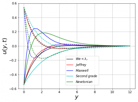
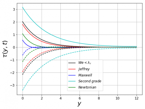
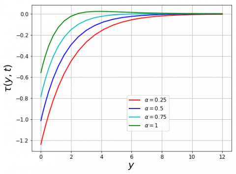
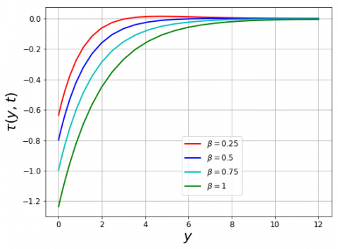
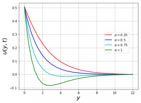
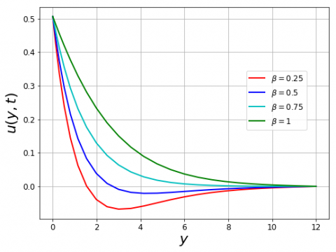
The accuracy of the solutions for different values of α, β, Nt, Ny are presented in Table 1 in terms of the maximum residual error and condition number. The condition number was computed using the python package ‘numpy.linalg.cond’. The results in Figure 1 are shown for two frequencies of oscillation and α=0.25, β=0.75, t=10, Re=0.1 and Ha=0.5. We consider the cases: We=1<λr=1.5, Jeffrey fluid (λr=1.2<We=1.5), Maxwell fluid (We=1.5, λr=0), second-grade fluid (We=0, λr=1.2) and Newtonian fluid. The figure shows the velocity and tangential shear stress profiles. In Figure 1a, the velocity profiles are plotted for special cases of the fractional Oldroyd–B fluid. In all cases, the oscillation of the fluid velocity decays as it approaches the boundary layer region. The fractional second-grade fluid has the lowest amplitude of oscillation, while the fractional Maxwell fluid has the highest amplitude. This result is in agreement with the study of Jamil et al. [26]. In Figure 1b, the shear stress profiles for fixed time t are plotted for special cases. This figure shows that the case We=0 (second-grade fluid) has the highest shear stress at the wall, while the case when λr=0 (Maxwell fluid) has the smallest shear stress. Figure 2 and Figure 3 illustrate the behaviour of the velocity and shear stress for different values of the fractional orders α and β. Figure 2 shows that as the order α increases, the shear stress decreases, while the net effect of increasing β is that the shear stress increases. In Figure 3, it can be seen that as β increases, the amplitude of oscillation becomes smaller while the amplitude becomes more significant as α increases. This result, in effect, shows that the likelihood of having a region of reverse flow close to the wall is less likely for fixed β, decreasing α and fixed α, increasing β. We remark that the degree of α is related to the relaxation time. Hence, the lack of reverse flow or small amplitude of oscillation for small values of α can be associated with the short memory of the fluid and slow response to shear stress.
Table 1. Residual and condition number for the problem in Section 4.1
|
(α,β) |
(Nt,Ny) |
Resu |
CNu |
Resτ |
CNτ |
|
(0.25,0.5) |
(5,5) |
4.1482e-16 |
203.5 |
1.3210e-15 |
17.35 |
|
|
(10,10) |
2.8511e-14 |
6.0310e+04 |
7.2893e-15 |
18.99 |
|
|
(15,15) |
1.3015e-07 |
6.1347e+11 |
1.7146e-07 |
8.6119e+04 |
|
(0.5,0.75) |
(5,5 ) |
9.0899e-16 |
313.1 |
1.1055e-15 |
24.02 |
|
|
(10,10 ) |
3.1403e-14 |
1.5079e+03 |
5.2698e-15 |
44.92 |
|
|
(15,15 ) |
3.5876e-07 |
5.6432e+11 |
1.2344e-06 |
4.1606e+06 |
|
(0.75,1) |
( 5,5 ) |
5.7333e-16 |
477.8 |
2.0091e-15 |
36.39 |
|
|
(10,10) |
4.8934e-14 |
4.3557e+04 |
7.8238e-15 |
104.4 |
|
|
(15,15) |
1.2859e-07 |
2.2473e+11 |
3.4619e-07 |
2.7625e+06 |
|
(1,1) |
(5,5 ) |
7.8409e-16 |
625.5 |
1.4658e-15 |
60.11 |
|
|
(10,10) |
7.6247e-14 |
7.0962e+04 |
1.7502e-14 |
236.8 |
|
|
(15,15 ) |
1.1289e-08 |
2.6527e+10 |
3.9879e-07 |
4.1076e+06 |
(a)
(b)
Figure 1. Velocity and shear stress of special cases of the fractional Oldroyd-B fluid with ω=70+nπ/2
(a)
(b)
Figure 2. Variation of the tangential shear stress profiles with ω=10+π/2 for (a) different α with β=1 and (b) different β with α=0.25
(a)
(b)
Figure 3. Velocity profiles with ω=10+π/2 for: (a) different α with β=1 and (b) different β with α=0.25
4.2 The non-isothermal flow of an Oldroyd–B fluid
Here we consider the unsteady non–isothermal flow of a generalized Oldroyd–B fluid. The thermal property of the fluid (γ), the specific heat (c) and the thermal conductivity (k) are constant and isotropic, except the viscosity which is assumed to be temperature-dependent with reference viscosity, μ0. We use [27]
$\mu(T)=\frac{\mu_{0}}{1+\gamma\left(T-T_{0}\right)}$ (50)
to model the non-isothermal viscosity. The system of equations describing the conservation of momentum Eq. (6) [Ha=0], the shear stress Eq. (7), and the energy equation are given as [28, 29]:
$R e\left[\frac{\partial u}{\partial t}+W e^{\alpha} \frac{\partial^{\alpha+1} u}{\partial t^{\alpha+1}}\right]-\left[\frac{\partial u}{\partial y} \frac{\partial}{\partial y}\left(\frac{1}{1+\theta_{e} \theta}\right)+\lambda_{r}^{\beta} \frac{\partial^{\beta+1} u}{\partial t^{\beta} \partial y} \frac{\partial}{\partial y}\left(\frac{1}{1+\theta_{e} \theta}\right)+\frac{1}{1+\theta_{e} \theta} \frac{\partial^{2} u}{\partial y^{2}}+\frac{1}{1+\theta_{e} \theta} \frac{\partial^{\beta+2} u}{\partial t^{\beta} \partial y^{2}}\right]=0$ (51)
$R e\left[\frac{\partial \theta}{\partial t}+W e^{\alpha} \frac{\partial^{\alpha+1} \theta}{\partial t^{\alpha+1}}\right]-\frac{1}{\operatorname{Pr}}\left[\frac{\partial^{2} \theta}{\partial y^{2}}+W e^{\alpha} \frac{\partial^{\alpha+2} \theta}{\partial t^{\alpha} \partial y^{2}}\right]-E c\left[\frac{1}{1+\theta_{e} \theta}\left(\frac{\partial u}{\partial y}\right)^{2}+\frac{\lambda_{r}^{\beta}}{1+\theta_{e} \theta} \frac{\partial^{\beta+1} u}{\partial t^{\beta} \partial y} \frac{\partial u}{\partial y}\right]=0$ (52)
$\left[1+W e^{\alpha} \frac{\partial^{\alpha}}{\partial t^{\alpha}}\right] \tau=\frac{1}{1+\theta_{e} \theta}\left[\frac{\partial u}{\partial y}+\lambda_{r}^{\beta} \frac{\partial^{\beta+1} u}{\partial t^{\beta} \partial y}\right]$ (53)
where, θe=γΔT, the temperature ratio, $E c=\mathbf{U}_{0}^{2}(c \Delta T)^{-1}$, the Eckert number, Pr=cμ0 k-1, the reference Prandtl number, θ=(T-T0)ΔT-1, the dimensionless temperature are dimensionless parameters. The initial and boundary conditions are given as in Eq. (45) and Eq. (46) and
$\theta(y, 0)=\frac{\partial}{\partial t} \theta(y, 0)=0 \forall y>0$ (54)
$\theta(0, t)=1, \quad \theta(y, t)=0$ as $y \rightarrow \infty, t>0$ (55)
We seek a solution in the form of Eq. (22) for each dependent variable and apply the quasi–linearization method to linearize the system of equations (see Bellman and Kalaba [30], Motsa et al. [31]):
$\begin{aligned}\left[\operatorname{Re}\left[\left(\mathrm{D}_{t}^{1} \otimes I_{y}\right)+W e^{\alpha}\left(D_{t}^{\alpha+1} \otimes I_{y}\right)\right]+a_{0 r}\left(I_{t} \otimes D_{y}^{2}\right)\right.\\+& a_{1 r}\left(I_{t} \otimes \mathrm{D}_{y}\right) \\+a_{2 r}\left(\mathrm{D}_{t}^{\beta} \otimes \mathrm{D}_{y}^{2}\right)+a_{3 r}\left(\mathrm{D}_{t}^{\beta}\right.& \\\left.\left.\otimes \mathrm{D}_{y}^{1}\right)\right] \operatorname{vec}\left(\vec{u}_{r+1}\right) \\+\left[a_{4 r}\left(I_{t} \otimes \mathrm{D}_{y}^{1}\right)\right.& \\\left.+a_{5 r}\left(I_{t} \otimes I_{y}\right)\right] \operatorname{vec}\left(\vec{\theta}_{r+1}\right) &=v e c\left(\vec{R}_{1 r}\right) \end{aligned}$ (56)
$\left[\operatorname{Re}\left(\mathrm{D}_{t}^{1} \otimes I_{y}\right)+\operatorname{Re} W e^{\alpha}\left(\mathrm{D}_{t}^{\alpha+1} \otimes I_{y}\right)-\frac{1}{\operatorname{Pr}}\left(I_{t} \otimes \mathrm{D}_{y}^{2}\right)\right.$
$-\frac{W e^{\alpha}}{\operatorname{Pr}}\left(\mathrm{D}_{t}^{\alpha} \otimes \mathrm{D}_{y}^{2}\right)+b_{2 r}\left(I_{t}\right.$$\left.\left.\otimes I_{y}\right)\right] \operatorname{vec}\left(\vec{\theta}_{r+1}\right)$
$+\left[b_{0 r}\left(I_{t} \otimes \mathrm{D}_{y}^{1}\right)+b_{1 r}\left(\mathrm{D}_{t}^{\beta}\right.\right.$$\left.\left.\otimes \mathrm{D}_{y}^{1}\right)\right] \operatorname{vec}\left(\vec{u}_{r+1}\right)=\operatorname{vec}\left(\vec{R}_{2 r}\right)$ (57)
Table 2. Residuals for the dependent variables in the problem in Section 4.2
|
(α,β) |
(Nt,Ny) |
Resu |
Resθ |
Resτ |
|
(0.25,0.5) |
(7,10) |
2.1518e-14 |
1.0823e-13 |
9.8749e-16 |
|
|
(10,15) |
1.7957e-13 |
6.2928e-13 |
6.8437e-15 |
|
|
(12,20) |
2.0137e-12 |
5.9289e-12 |
3.9240e-14 |
|
(0.5,0.75) |
(7,10) |
3.2932e-14 |
1.7114e-13 |
1.0634e-15 |
|
|
(10,15) |
4.0798e-13 |
9.5568e-13 |
4.3160e-15 |
|
|
(12,20) |
5.1502e-12 |
8.9247e-12 |
4.9766e-14 |
|
(0.75,1) |
(7,10) |
4.4381e-14 |
1.3593e-13 |
2.2664e-15 |
|
|
(10,15) |
1.1795e-12 |
1.3475e-12 |
2.0567e-14 |
|
|
(12 ,20) |
1.4751e-11 |
1.9498e-11 |
3.6492e-14 |
|
(1,1) |
(7,10) |
7.6759e-14 |
1.3427e-13 |
3.5037e-15 |
|
|
(10,15) |
2.0559e-12 |
3.0306e-12 |
1.7538e-14 |
(a)
(b)
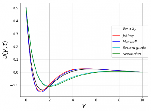
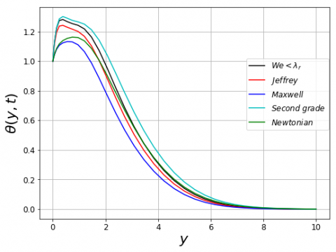
Figure 4. Velocity and temperature profiles for non-isothermal flow of the special cases of the fractional Oldroyd-B fluid
(a)
(b)
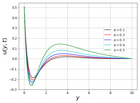
Figure 5. Velocity profiles of the non-isothermal flow for (a) β= 0.5 and (b) α=0.1
Table 2 shows the maximum residual error for 0≤t≤10 for different values of α and β. In Figure 4, the velocity and temperature profiles are illustrated for the special cases of the fractional Oldroyd–B fluid with α=0.25, β=0.5, Re=1.1, Pr=5, Ec=0.2, θe=0.33 and ω=10+π/2. We consider the cases: We=0.2<λr=1.5, Jeffrey fluid (λr=1.2<We=1.5), Maxwell fluid (We=1.5, λr=0), second-grade fluid (We=0, λr=1.2) and Newtonian fluid. It can be seen that, as in Section 4.1, the second-order fluid has the smallest amplitude while the Maxwell fluid has the highest oscillation amplitude. However, for the temperature profiles, the Maxwell fluid reaches its thermal boundary layer region quicker than the other fluids, and the second-grade fluid has the most extensive thermal boundary layer. Figure 4b also show increased temperature close to the wall. The study of Ishfaq et al. [28] attributes this behaviour to the accumulation of energy in the fluid particles in the vicinity of the wall because the viscous effect is profoundly felt in this region. The effects of different orders of derivatives are shown in Figure 5. Unlike the problem in Section 4.1, where velocity profiles are either strictly increasing or decreasing functions of α and β, in this flow, the velocity profiles intersect. We ascribe this behaviour to the coupling effect and non–isothermic nature of the fluid.
In this study, efficient and accurate numerical solutions for unsteady and unidirectional flows of generalized Oldroyd–B fluids have been obtained using the shifted Chebyshev polynomials of the first kind as the basis function. The two problems presented have a varying degree of complexity, which are mainly non–linearity and coupling. The accuracy of the solutions was investigated through the calculation of the residual error norm. The condition number of the discretization matrices was also presented for various values of the orders of derivatives and truncation of the Chebyshev series. The effects of the fractional-order derivatives in the constitutive equation of the Oldroyd–B fluid on shear stress and velocity are also discussed. We found that small values of the order of the relaxation term can be used to model the flow of viscoelastic fluid with short-term memory and slow response to shear force. Since many fluid dynamics problems exist on complex geometries, improvement can be made to accommodate problems with complex geometries.
B0 the applied magnetic field, N⋅s / C⋅m
c specific heat capacity, J/ K/ kg
Ec Eckert number
eij stress tensor, N/m2
Ha Hartmann number
k thermal conductivity, W/ m⋅K
Pr reference Prandtl number
Re Reynolds number
U0 reference velocity, m/s
We Weissenberg number
Greek symbols
α,β fractional orders
θe temperature ratio
λ relaxation time, s
λr retardation time, s/ dimensionless retardation time
μ viscosity, kg/m/s
μ0 reference viscosity, kg/m/s
ρ fluid density, kg/m3
σ electrical conductivity, S/m
τ shear stress, N/m2
ω frequency of oscillation, s-1
The vectors R1r and R2r in Eq. (56) and Eq. (57) are defined as
$\begin{aligned} R_{1 r}=a_{0 r} \frac{\partial^{2} u_{r}}{\partial y^{2}}+& a_{1 r} \frac{\partial u_{r}}{\partial y}+a_{2 r} \frac{\partial^{\beta+2} u_{r}}{\partial t^{\beta} \partial y^{2}} \\ &+a_{3 r} \frac{\partial^{\beta+1} u_{r}}{\partial t^{\beta} \partial y}+a_{4 r} \frac{\partial \theta_{r}}{\partial y}+a_{5 r} \theta_{r} \\ &-N u_{r} \end{aligned}$ (58)
where,
$\begin{aligned} N u_{r}=-\frac{\partial u_{r}}{\partial y} \frac{\partial}{\partial y}\left(\frac{1}{1+\theta_{e} \theta_{r}}\right)-\lambda_{r}^{\beta} \frac{\partial^{\beta+1} u_{r}}{\partial t^{\beta} \partial y} \frac{\partial}{\partial y}\left(\frac{1}{1+\theta_{e} \theta_{r}}\right) \\ &-\frac{1}{1+\theta_{e} \theta_{r}} \frac{\partial^{2} u_{r}}{\partial y^{2}}-\frac{1}{1+\theta_{e} \theta_{r}} \frac{\partial^{\beta+2} u_{r}}{\partial t^{\beta} \partial y^{2}} \end{aligned}$
$a_{0 r}=-\left(1+\theta_{e} \theta_{r}\right)^{-1}, \quad a_{1 r}=\theta_{e}\left(1+\theta_{e} \theta_{r}\right)^{-2} \frac{\partial \theta_{r}}{\partial y}$
$a_{2 r}=-\left(1+\theta_{e} \theta_{r}\right)^{-1}$$a_{3 r}=\theta_{e} \lambda_{r}^{\beta}\left(1+\theta_{e} \theta_{r}\right)^{-2} \frac{\partial \theta_{r}}{\partial y}$
$a_{4 r}=\theta_{e}\left(1+\theta_{e} \theta_{r}\right)^{-2}\left(\frac{\partial u_{r}}{\partial y}+\lambda_{r}^{\beta} \frac{\partial^{\beta+1} u_{r}}{\partial t^{\beta} \partial y}\right)$
$\begin{aligned} a_{5 r}=-2 \theta_{e}^{2}\left(1+\theta_{e} \theta_{r}\right)^{-3}\left(\frac{\partial \theta_{r}}{\partial y} \frac{\partial u_{r}}{\partial y}+\lambda_{r}^{\beta} \frac{\partial \theta_{r}}{\partial y} \frac{\partial^{\beta+1} u_{r}}{\partial t^{\beta} \partial y}\right) \\ &+\theta_{e}\left(1+\theta_{e} \theta_{r}\right)^{-2}\left(\frac{\partial^{2} u_{r}}{\partial y^{2}}+\frac{\partial^{\beta+2} u_{r}}{\partial t^{\beta} \partial y^{2}}\right) \end{aligned}$
and
$R_{2 r}=b_{0 r} \frac{\partial u_{r}}{\partial y}+b_{1 r} \frac{\partial^{\beta+1} u_{r}}{\partial t^{\beta} \partial y}+b_{2 r} \theta_{r}-N \theta r$ (59)
Here,
$N \theta_{r}=-E c\left[\frac{1}{1+\theta_{e} \theta_{r}}\left(\frac{\partial u_{r}}{\partial y}\right)^{2}+\frac{\lambda_{r}^{\beta}}{1+\theta_{e} \theta_{r}} \frac{\partial^{\beta+1} u_{r}}{\partial t^{\beta} \partial y} \frac{\partial u_{r}}{\partial y}\right]$
$b_{0 r}=-2 E c\left(1+\theta_{e} \theta_{r}\right)^{-1} \frac{\partial u_{r}}{\partial y}-\lambda_{r}^{\beta}\left(1+\theta_{e} \theta_{r}\right)^{-1} \frac{\partial^{\beta+1} u_{r}}{\partial t^{\beta} \partial y}$
$b_{1 r}=-\lambda_{r}^{\beta}\left(1+\theta_{e} \theta_{r}\right)^{-1} \frac{\partial u_{r}}{\partial y}$
$b_{2 r}=\theta_{e}\left(1+\theta_{e} \theta_{r}\right)^{-1}\left(E c\left(\frac{\partial u_{r}}{\partial y}\right)^{2}+\lambda_{r}^{\beta} \frac{\partial^{\beta+1} u_{r}}{\partial t^{\beta} \partial y} \frac{\partial u_{r}}{\partial y}\right)$
[1] Oldroyd, J. (1958). Non-Newtonian effects in steady motion of some idealized elastico-viscous liquids. Proceedings of the Royal Society London Series A, 245: 278-297.
[2] Maxwell, J.C. (2003). On the dynamical theory of gases: The Kinetic Theory of Gases: An anthology of classic papers with historical commentary. World Scientific, 197-261.
[3] Tarasov, V.E. (2013). Review of some promising fractional physical models. International Journal of Modern Physics B, 27(9): 1330005. http://dx.doi.org/10.1142/S0217979213300053
[4] Jamil, M., Khan, N., Zafar, A. (2011). Translational flows of an Oldroyd-B fluid with fractional derivatives. Computers & Mathematics with Applications, 62(3): 1540-1553. http://dx.doi.org/10.1016/j.camwa.2011.03.090
[5] Bazhlekova, E., Bazhlekov, I. (2017). Stokes’ first problem for viscoelastic fluids with a fractional Maxwell model. Fractal and Fractional, 1(1): 7. http://dx.doi.org/10.3390/fractalfract1010007
[6] Le Roux, C. (2014). On flows of viscoelastic fluids of Oldroyd type with wall slip. Journal of Mathematical Fluid Mechanics, 16(2): 335-350. http://dx.doi.org/10.1007/s00021-013-0159-9
[7] Wang, Q. (2006). Numerical solutions for fractional KdV–Burgers equation by Adomian decomposition method. Applied Mathematics and Computation, 182(2): 1048-1055. http://dx.doi.org/10.1016/j.amc.2006.05.004
[8] Diethelm, K., Ford, N.J., Freed, A.D. (2002). A predictor-corrector approach for the numerical solution of fractional differential equations. Nonlinear Dynamics, 29: 3-22.
[9] Erjaee, G., Taghvafard, H., Alnasr M. (2011). Numerical solution of the high thermal loss problem presented by a fractional differential equation. Communications in Nonlinear Science and Numerical Simulation, 169(3): 1356-1362. http://dx.doi.org/10.1016/j.cnsns.2010.06.031
[10] El-Sayed, A., El-Kalla, I., Ziada, E. (2010). Analytical and numerical solutions of multiterm nonlinear fractional orders differential equations. Applied Numerical Mathematics, 60(8): 788-797. http://dx.doi.org/10.1016/j.apnum.2010.02.007
[11] Momani, S., Odibat, Z. (2007) Comparison between the homotopy perturbation method and the variational iteration method for linear fractional partial differential equations. Computers & Mathematics with Applications, 54(7-8): 910-919. http://dx.doi.org/10.1016/j.camwa.2006.12.037
[12] Momani, S., Odibat, Z. (2007). Homotopy perturbation method for nonlinear partial differential equations of fractional order. Physics Letters A, 365(5-6): 345-350. http://dx.doi.org/10.1016/j.physleta.2007.01.046
[13] Doha, E., A. Bhrawy, A., Ezz-Eldien, S. (2011). Efficient Chebyshev spectral methods for solving multiterm fractional orders differential equations. Applied Mathematical Modelling, 35(12): 5662-5672. http://dx.doi.org/10.1016/j.apm.2011.05.011
[14] Atabakzadeh, M., Akrami, M., Erjaee, G. (2013). Chebyshev operational matrix method for solving multi-order fractional ordinary differential equations. Applied Mathematical Modelling, 37(20-21): 8903-8911. http://dx.doi.org/10.1016/j.apm.2013.04.019
[15] Liu, J., Li, X., Wu, L. (2016). An operational matrix of fractional differentiation of the second kind of Chebyshev polynomial for solving multiterm variable order fractional differential equation. Mathematical Problems in Engineering. http://dx.doi.org/10.1155/2016/7126080
[16] Benattia, M.E., Belghaba, K. (2017). Numerical solution for solving fractional differential equations using shifted Chebyshev wavelet. General Letters in Mathematics, 3: 101-110.
[17] Bhrawy, A.H., Alghamdi, M.A. (2013). The operational matrix of Caputo fractional derivatives of modified generalized Laguerre polynomials and its applications. Advances in Difference Equations, 307. http://dx.doi.org/10.1186/1687-1847-2013-307
[18] Baseri, A., Babolian, E., Abbasbandy, S. (2017). Normalized Bernstein polynomials in solving space-time fractional diffusion equation. Advances in Difference Equations, 346. http://dx.doi.org/10.1186/s13662-017-1401-1
[19] Podlubny, I. (1998). Fractional differential equations: an introduction to fractional derivatives, fractional differential equations, to methods of their solution and some of their applications. Elsevier.
[20] Atangana, A. (2017). Fractional operators with constant and variable order with application to geo-hydrology. Academic Press.
[21] Abramowitz, M., Stegun, I.A. (1965). Handbook of mathematical functions: with formulas, graphs, and mathematical tables, Courier Corporation.
[22] Ahmadi Darani, M., Saadatmandi, A. (2017). The operational matrix of fractional derivative of the fractional-order Chebyshev functions and its applications. Computational Methods for Differential Equations, 5: 67-87.
[23] Ahmadi Darani, M., Nasiri, M. (2013). A fractional type of the Chebyshev polynomials for approximation of solution of linear fractional differential equations. Computational Methods for Differential Equations, 1: 96-107.
[24] Shao, W., Wu, X., Chen, S. (2012). Chebyshev tau meshless method based on the integration–differentiation for biharmonic-type equations on irregular domain. Engineering Analysis with Boundary Elements, 36(12): 1787-1798. http://dx.doi.org/10.1016/j.enganabound.2012.06.005
[25] Bhrawy, A.H. (2016). A highly accurate collocation algorithm for 1+1 and 2+1 fractional percolation equations. Journal of Vibration and Control, 22(9): 2288-2310. http://dx.doi.org/10.1177/1077546315597815
[26] Jamil, M., Khan, A.N., Shahid, N. (2013). Fractional magnetohydrodynamics Oldroyd-B fluid over an oscillating plate. Thermal Science, 17(4): 997-1011. http://dx.doi.org/10.2298/TSCI110731140J
[27] Lai, F., Kulacki, F. (1990). The effect of variable viscosity on convective heat transfer along a vertical surface in a saturated porous medium. International Journal of Heat and Mass Transfer, 33(5): 1028-1031. http://dx.doi.org/10.1016/0017-9310(90)90084-8
[28] Ishfaq, N., Khan, W., Khan, Z. (2017). The Stokes’ second problem for nanofluids. Journal of King Saud University-Science. 31(1): 61. http://dx.doi.org/10.1016/j.jksus.2017.05.001
[29] Zhao, J., Zheng, L., Zhang, X., Liu, F. (2016). Unsteady natural convection boundary layer heat transfer of fractional Maxwell viscoelastic fluid over a vertical plate. International Journal of Heat and Mass Transfer, 97: 760-766. http://dx.doi.org/10.1016/j.ijheatmasstransfer.2016.02.059
[30] Bellman, R.E., Kalaba, R.E. (1965). Quasilinearization and nonlinear boundary-value problems.
[31] Motsa, S.S., Magagula, V., Sibanda, P. (2014). A bivariate Chebyshev spectral collocation quasilinearization method for nonlinear evolution parabolic equations. The Scientific World Journal. http://dx.doi.org/10.1155/2014/581987